Introduction to scikit-learn (sklearn)

Scikit-learn, also known as sklearn, is the most usable and robust Machine Learning Python library. It allows you to use classification, regression, clustering, dimensionality reduction, and other helpful ML and statistical modeling algorithms for predictive data analysis without the need to code them yourself. Scikit-learn integrates well with many other Python libraries, such as Matplotlib and Plotly, NumPy for array vectorization, Pandas DataFrames, SciPy, and many more. This article will cover the sklearn and basic statistical modeling algorithms you can use by including this module in your Python programs.

Best Machine Learning Books for Beginners and Experts

As Machine Learning becomes more and more widespread, both beginners and experts need to stay up to date on the latest advancements. For beginners, check out the best Machine Learning books that can help to get a solid understanding of the basics. For experts, reading these books can help to keep pace with the ever-changing landscape. In either case, a few key reasons for checking out these books can be beneficial.

First, they provide a comprehensive overview of the subject matter, mainly about Machine Learning algorithms. Second, they offer insights from leading experts in the field. And third, they offer concrete advice on how to apply Machine Learning concepts in real-world scenarios. As Machine Learning continues to evolve, there’s no doubt that these books will continue to be essential resources for anyone with prior knowledge looking to stay ahead of the curve.

Installation of sklearn

scikit-learn is a Python module for machine learning built on top of SciPy and is distributed under the 3-Clause BSD license. David Cournapeau initially developed Sklearn as a Google Summer of Code project in 2007. Later many other professionals contributed to this project and took it to another level. The scikit-learn project is hosted on GitHub, where anyone can contribute.

The most common and popular way of installing the scikit learn module on your system is by using the pip command.

#installing scikit learn module
pip install scikit-learn

Once you have installed the sklearn module, you can check its version from your Python code:

# importing the module
import sklearn
# printing the version
print(sklearn.__version__)

Output:

You can update the existing installed sklearn module on your system by typing the following command:

pip install --upgrade scikit-learn

Data pre-processing in the scikit learn module

The data we usually deal with is stored in so-called raw format, and we need to process it to make it suitable for ML algorithms. This process is called preprocessing, and it allows us to check missing values, noisy data, and other inconsistencies before training the ML model. This section will use the scikit learn module to preprocess the data.

For example, let’s say that we have the following dataset:

# Importing the required libraries
import numpy as np
# creating numpy dataset
data = np.array([
   [3.4, -1.8, 5.1],
   [-4.5, 2.4, 3.3],
   [3.5, -7.2, 5.1],
   [5.7, 2.5, -2.8]]
)
# printing
print(data)

Output:

Now, let’s apply different methods to preprocess this dataset.

Binarization of dataset

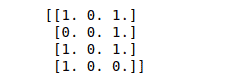
Binarization is the technique used to convert numerical values into boolean values. This process will convert all negative values to zero (False) and positive values to 1 (True).

# importing the module
from sklearn import preprocessing
# converting to binary dataset
binary_data = preprocessing.Binarizer().transform(data)
# printing
print(binary_data)

Output:

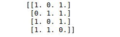
We can also specify the threshold value for the binary conversion. By default, the threshold value is 0: any values above the threshold value will be considered 1, and below will be considered 0.

# converting to binary dataset threshold value 3
binary_data = preprocessing.Binarizer(threshold=3).transform(data)
# printing
print(binary_data)

Output:

Standardize a dataset along any axis

To standardize a dataset along any axis, you need to use the preprocessing.scale() method of the scikit learn module. This method eliminates the mean from the feature vector so that every feature is centered on zero, and the standard deviation will be 1.

Do not use scale unless you know what you are doing. A common mistake is to apply it to the entire data before splitting into training and test sets (independent and dependent variables). This will bias the model evaluation because information would have leaked from the test set to the training set.

scikit-learn.org

# Mean and the standard deviation of the dataset
print("Mean =", data.mean(axis=0))
print("Std-deviation =", data.std(axis=0))

Output:

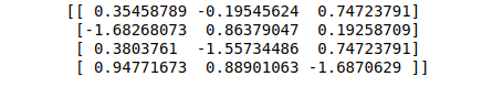
Let’s scale our data so that every feature is centered at zero and the standard deviation becomes 1.

# scaling dataset
data_scaled = preprocessing.scale(data)
# printing mean and deviation
print("Mean_removed =", data_scaled.mean(axis=0))
print("Stddeviation_removed =", data_scaled.std(axis=0))

Output:

After scaling, the data looks like this:

# printing scaled data
print(data_scaled)

Output:

Scaling the dataset

The preprocessing.MinMaxScaler class is used to scale the feature vectors. The scaling of feature vectors is essential to reduce features’ influence on the ML model output. We can specify the range for scaling as shown below:

# specifiying  range for scalling
data_scaled = preprocessing.MinMaxScaler(feature_range=(0,1))
# scalling the dataset
data_scaled = data_scaled.fit_transform(data)
# printing scaled dataset
print ("scaled data is :\n", data_scaled)

Output:

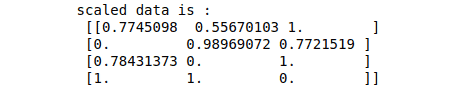
Note that the data has been scaled between 0 and 1. Similarly, we can specify other ranges, and the elements will be arranged accordingly.

Normalization techniques

In preprocessing, normalization is used to modify the feature vectors. Sometimes, it is required to measure the feature vectors using a common scale. The scikit learn module provides two different types of normalization techniques.

l1 normalization or Least Absolute Deviations technique modifies the value in such a way that the sum of the absolute values always remains up to 1 in each row, for example:

# normalizing the data using Least Absolute Deviations
l1_normalization = preprocessing.normalize(data, norm='l1')
# printing
print("L1 normalized data is :\n", l1_normalization)

Output:

We can verify that the sum of absolute values in each of the rows is 1:

# finding sum
Sum=[sum(abs(i)) for i in l1_normalization]
# printing
print (Sum)

Output:

l2 normalization or Least Squares modifies the value so that the sum of the squares always remains up to 1 in each row. Let us apply this method of normalization to our data:

# l2 normalization technique
l2_normalization = preprocessing.normalize(data, norm='l2')
# printing
print("L1 normalized data is :\n", l2_normalization)

Output:

We can verify that the sum of squares in each row equals 1.

# finding sum of squares
Sum=[sum(i*i) for i in l2_normalization]
# printing
print (Sum)

Output:

Supervised Machine Learning algorithms

There are three Machine Learning algorithms: supervised machine learning, unsupervised machine learning, and reinforcement learning. The scikit learn module is one of the most popular modules for Machine Learning as it provides various built-in ML algorithms, which we will discuss in this section.

Before applying these algorithms, let’s load the dataset and split it into the training and testing part. We will use the Iris dataset (one of the most popular ML datasets for education).

We can import the Iris dataset from the datasets module of scikit learn.

# importing the dataset
from sklearn.datasets import load_iris
# loading dataset
iris = load_iris()

Let’s divide the dataset into features and target variables (outputs) and print them out:

# input and target variables
Inputs = iris.data
Target= iris.target
# getiing features names and target variables
feature_names = iris.feature_names
target_names = iris.target_names
# printing
print("Feature names:", feature_names)
print("Target names:", target_names)

Output:

The next essential feature in the scikit learn module allows us to split datasets into the training and testing parts. The training is used to train the model, and the testing is used to test/validate the model’s predictions.

# importing the module
from sklearn.model_selection import train_test_split
# splitting the dataset into testing and training part
X_train, X_test, y_train, y_test = train_test_split(
   Inputs, Target, test_size = 0.25)

The train_test_split method will randomly assign 25% of the data to testing and 75% to the training part.

Support Vector Machine (SVM) algorithm

Support Vector Machines (SVM), also known as Support Vector Classification, is a supervised and linear regression ML algorithm used to solve classification problems. The Support Vector Regression (SVR) algorithm is a subset of SVM algorithms that uses the same ideas to tackle regression problems. You can learn more about the SVM algorithm from the Support Vector Machines using Python article.

Here we will use the scikit learn module to import the built-in SVM algorithm and apply it to our dataset:

# importing module
from sklearn.svm import SVC
# initializing SVM
SVC_classifier = SVC(kernel = 'linear',gamma = 'scale', shrinking = False,)
SVC_classifier.fit(X_train,y_train )

The SVM takes the following parameters:

• kernel : This parameter specifies the type of kernel to be used in the algorithm. We can choose from the linear, poly, rbf, sigmoid, and precomputed. The default value of kernel is rbf.
• gamma: It is the kernel coefficient for rbf, poly and sigmoid kernels.
• shrinking : This parameter represents that whether we want to use the shrinking heuristic or not, the Default value is True.
• probability: This parameter enables or disables probability estimates. The default value is False.
• max_iter: parameter represents the maximum number of iterations within the solver. Its default value is -1 , which means there is no limit on the number of iterations.
• random_state: This parameter represents the seed of the pseudo-random number generated, used while shuffling the data.

Once the training is complete, we can predict the outputs by providing only the inputs.

# model predictions
SVM_predictions = SVC_classifier.predict(X_test)

# printing prodictions
print(SVM_predictions)

Output:

K-nearest neighbors (KNN)

KNN is a supervised, non-parametric, and lazy learning algorithm that handles classification problems. It is a lazy learner because it doesn’t learn a discriminative function from the training data but memorizes the training dataset instead. There is no trained model for KNN. Each time we run the algorithm, it processes the entire model to provide the output. You can learn more about the KNN algorithm from the Implementing KNN Algorithm using Python article.

Here we will use the KNN algorithm from the scikit learn module and apply it to our dataset:

# importing KNN algorithm
from sklearn.neighbors import KNeighborsClassifier
# K value set to be 5
KNN_classifer = KNeighborsClassifier(n_neighbors=5)
# fitting the model on training dataset
KNN_classifer.fit(X_train,y_train)

Once the training is complete, we can provide the test dataset to predict the outputs.

# predicting 
KNN_predictions = KNN_classifer.predict(X_test)
# print
print(KNN_predictions)

Output:

Decision Tree algorithm

A Decision Tree is a Supervised ML algorithm used to categorize or predict outcomes based on the previous dataset. It is a tree-structured classifier where internal nodes represent the features of a dataset, branches represent the decision rules, and each leaf node represents the decision outcome. You can read more about the Decision Tree algorithm from the Implementing Decision Tree Using Python article.

# importing decision tree
from sklearn import tree
# initializaing the decision tree classifier
DT_classifier = tree.DecisionTreeClassifier()
# training the tree
DT_classifier.fit(X_train,y_train)

The decision tree classifier takes the following parameters:

• criterion: represents the function to measure the quality of a split. You can choose gini or entropy. By default, the value is gini.
• splitter: tells the model which strategy (best or random) to choose while splitting the data. By default, the value is best.
• max_depth: this parameter defines the maximum depth of the tree. The default value is None which means the nodes will expand until all leaves are pure or until all leaves contain less than min_smaples_split samples.
• min_samples_split: parameter provides the minimum number of samples required to split an internal node. The default value is 2.
• min_samples_leaf: parameter provides the minimum number of samples required at a leaf node. The default value is 1.
• min_weight_fraction_leaf: is used to get the minimum weighted fraction of the sum of weights required to be at a leaf node. The default value is 0.
• max_features: defines the number of features of the model to be considered when looking for the best split.
• max_leaf_nodes: this parameter will limit a tree’s growth to the maximum leaf nodes.
• min_impurity_decrease: this value works as a criterion for a node to split.
• min_impurity_split: represents the threshold for early stopping in tree growth.

Once the training is complete, we can predict the output by providing the testing data.

# predicting outputs
DT_predictions = DT_classifier.predict(X_test)
# printing
print(DT_predictions)

Output:

The Decision Tree algorithm can also be used for regression problems:

# regression problem using decision tree
DT_regressor = tree.DecisionTreeRegressor()
# training
DT_regressor.fit(X_train, y_train)
# predicting
DTR_predictions = DT_regressor.predict(X_test)
# printing
print(DTR_predictions)

Output:

Notice that the output values are not integer values anymore.

Random Forest algorithm

The concept of the Random Forest Algorithm is based on ensemble learning. Ensemble learning is a general meta-approach in Machine Learning that seeks better predictive performance by combining the predictions from multiple models. In simple words, It involves fitting many different model types on the same data and using another model to learn the best way to combine the predictions. So, Random Forest Algorithm combines predictions from decision trees and selects the best prediction among those trees. You can learn more about the working of a Random Forest Tree from the Implementation of Random Forests algorithm using Python article.

Like the Decision Tree algorithm, we can do classification and regression using the Random Forest Tree. Let’s import the Random forest model from the scikit learn module and train it on our dataset:

# importing random forest
from sklearn.ensemble import RandomForestClassifier
# training the model
RF_classifier = RandomForestClassifier(n_estimators = 50)
RF_classifier.fit(X_train, y_train)

Once the training is complete, we can provide the testing data to test our algorithm:

# predictions
RF_predictions = RF_classifier.predict(X_test)
# printing
RF_predictions

Output:

Similarly, we can also apply the Random Forest algorithm for regression problems.

# importing random forest
from sklearn.ensemble import RandomForestRegressor
# training the model
RF_regressor = RandomForestRegressor(n_estimators = 50)
RF_regressor.fit(X_train, y_train)
#predictions
RFR_predictions = RF_regressor.predict(X_test)
print(RFR_predictions)

Output:

Notice that we get continuous values as an output.

Naive Bayes algorithm

The Naive Bayes classification algorithm is a probabilistic classifier and belongs to Supervised learning. It is based on probability models that incorporate strong independence assumptions. The independence assumptions often do not have an impact on reality. Therefore they are considered naive. You can read more about the working of Naive Bayes classification from the Implementing Naive Bayes Classification using Python article.

There are several Naive Bayes algorithm implementations (classifiers) available in the sklearn module:

• Gaussian Naive Bayes: assumes that the data from each label is drawn from a simple Gaussian distribution.
• Multinomial Naive Bayes: assumes that the features are drawn from a simple Multinomial distribution.
• Bernouli Naive Bayes: The assumption in this model is that the features are binary (0 and 1).
• Complement Naive Bayes: was designed to correct the severe assumptions made by Multinomial Bayes classifier. This kind of classifier is suitable for imbalanced data sets.

We will use the Gaussian Naive Bayes classifier to classify the testing data. Let’s train our model using the training dataset:

# import Gaussian Naive Bayes classifier
from sklearn.naive_bayes import GaussianNB
# create a Gaussian Classifier
NB_classifier = GaussianNB()
# training the model
NB_classifier.fit(X_train, y_train)
# testing the model
NB_predictions = NB_classifier.predict(X_test)
# printing
print(NB_predictions)

Output:

AdaBoost algorithm

Boosting methods incrementally build ensemble models. The main principle is to build the model incrementally by training each base model estimator sequentially. AdaBoost is one of the most successful boosting ensemble methods whose main key is in the way they give weights to the instances in the dataset. The algorithm needs to pay less attention to the instances while constructing subsequent models.

Let’s apply this classifier to our dataset:

# Importing the module
from sklearn.ensemble import AdaBoostClassifier
# adaBoost 
AB_classifier = AdaBoostClassifier(n_estimators = 50)
# training the model
AB_classifier.fit(X_train, y_train)

Once the training is complete, we can provide the testing data to predict the outputs.

# predicting the outputs
AB_predictions = AB_classifier.predict(X_test)
# printing
print(AB_predictions)

Output:

Similarly, we can apply the AdaBoost algorithm to regression problems:

# importing the module
from sklearn.ensemble import AdaBoostRegressor
# initializing the algorithm
AB_regressor = AdaBoostRegressor()
# training the model
AB_regressor.fit(X_train, y_train)
# prediting
ABG_predictions = AB_regressor.predict(X_test)
# print
print(ABG_predictions)

Output:

Gradient Tree Boosting algorithm

The Gradient Boosted Regression Trees (GRBT) algorithm is used for classification and regression problems. It is a generalization of boosting to arbitrary differentiable loss functions.

For creating a Gradient Tree Boost classifier, we need to import GradientBoostingClassifier from the scikit-learn module:

# Importing the GBC
from sklearn.ensemble import GradientBoostingClassifier
# initializing the model
GB_classifier = GradientBoostingClassifier(n_estimators = 70)
# training the modle
GB_classifier.fit(X_train, y_train)
# prediciting
GBC_predictions = GB_classifier.predict(X_test)
# printing
print(GBC_predictions)

Output:

For creating a regressor with the Gradient Tree Boost method, we have to import GradientBoostingRegressor from the scikit learn module:

# importing the module
from sklearn.ensemble import GradientBoostingRegressor
# initializing the model
GB_regressor = GradientBoostingRegressor()
# training the modle
GB_regressor.fit(X_train, y_train)
# prediciting
GBR_predictions = GB_regressor.predict(X_test)
# printing
print(GBR_predictions)

Output:

Unsupervised Machine Learning algorithms

Unsupervised Machine Learning is a technique that teaches machines to classify unlabeled or unclassified data. The idea here is to expose computers to large volumes of data to find common data items’ features and use them to categorize that data. You can learn more about Unsupervised Machine Learning from the Introduction to Unsupervised Machine Learning article.

We will use the digits dataset set from the scikit learn module to demonstrate Unsupervised Learning examples. Let’s import the dataset:

# importing datast from sklearn module
from sklearn.datasets import load_digits
# loading dataset
digits = load_digits()
#shape of the dataset
digits.data.shape

Output:

K-means clustering algorithm

The K-means clustering is the Unsupervised Learning algorithm that splits a dataset into K non-overlapping subgroups (clusters). It allows us to split the data into different groups or categories. You can learn more about the working of K-means clustering from the Implementation of K-means clustering algorithm using Python article.

Here we will just import the clustering model from the scikit learn module:

# importing the k-mean clustering
from sklearn.cluster import KMeans
# making 10 clusters
kmeans = KMeans(n_clusters = 10, random_state = 0)
Kmeans_clusters = kmeans.fit_predict(digits.data)

We can check the number of clusters by printing the shape of the kmeans model.

print(kmeans.cluster_centers_.shape)

Output:

Notice the shape is now 10, which means it has created 10 clusters as defined by us in the training part.

Hierarchical clustering algorithm

Hierarchical clustering is another Unsupervised Machine Learning algorithm used to group unlabeled datasets into a cluster. It develops the hierarchy of clusters in the form of a tree-shaped structure known as a dendrogram. You can learn more about hierarchical clustering from the Implementation of Hierarchical clustering using Python article.

Let’s first import the Hierarchical clustering algorithm from scikit learn and then apply it to our dataset:

# Importing the algorithm
from sklearn.cluster import AgglomerativeClustering
# calling the agglomerative algorithm
H_clustering = AgglomerativeClustering(n_clusters = 8, affinity = 'euclidean', linkage ='average')
# training the model on dataset
H_model = H_clustering.fit_predict(digits.data)

We know that Hierarchical clustering works based on the dendrogram. A dendrogram is a tree-like structure that stores each step of the Hierarchical algorithm execution process. In the Dendrogram plot, the x-axis shows all data points, and the y-axis shows the distance between them. We can also visualize the dendrogram using the scikit learn module.

# importing the required modules
import matplotlib.pyplot as plt
import scipy.cluster.hierarchy as sch
# graph size
plt.figure(1, figsize = (16 ,8))
# creating the dendrogram
dendrogram = sch.dendrogram(sch.linkage(digits.data, method  = "ward"))
# ploting graphabs
plt.title('Dendrogram')
plt.show()

Output:

Dimensional reduction using Principal Component Analysis (PCA)

Principal Component Analysis (PCA) is used for linear dimensionality reduction using the Singular Value Decomposition (SVD) of the data to project it to a lower-dimensional space. You can learn more about PCA from the Implementing Principal Component Analysis (PCA) using Python article.

Here we will use the PCA to decompose our dataset into 3 and 2 dimensions:

# importing the required PCA
from sklearn.decomposition import PCA
# PCA with 3 component
pca = PCA(n_components = 3)
# fitting the dataset
fit = pca.fit(digits.data)
# printing the three PCA components
print(("Explained Variance: %s") % (fit.explained_variance_ratio_))

Output:

To have two PCA components, we have to change the number of components to 2.

# PCA with 2 component
pca = PCA(n_components = 2)
# fitting the dataset
fit = pca.fit(digits.data)
# printing the three PCA components
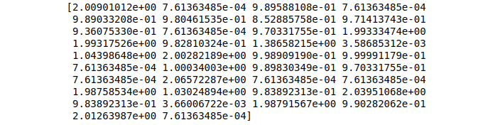
print(("Explained Variance: %s") % (fit.explained_variance_ratio_))

Output:

Once we have decomposed our dataset into 2 and 3 PCA components, we can easily visualize the dataset to see the relationship.

ML model evaluation methods

Model evaluation is essential to assess the efficacy of a model during the initial research phases, and it also plays a role in model monitoring. The model evaluation uses different metrics to understand an ML model’s accuracy and performance. Depending on the model type, there are various kinds of evaluating metrics. In this section, we will use some of these matrices to assess the performance of the models we built in the above section.

Evaluation of classification models

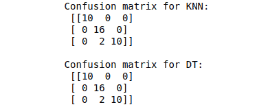
A confusion matrix is one of the available methods for calculating and evaluating any classification algorithm’s performance. It helps us calculate the accuracy, precision, f1-score, and recall of the classification model.

Let’s calculate the confusion matrix for the KNN and Decision Tree classifier built in the above sections.

# Making the Confusion Matrix
from sklearn.metrics import confusion_matrix
# providing actual and predicted values of knn
cm_KNN = confusion_matrix(y_test, KNN_predictions)
# confusion matrix for decision tree
cm_DT= confusion_matrix(y_test, DT_predictions)
# printing 
print("Confusion matrix for KNN: \n", cm_KNN)
print("\nConfusion matrix for DT: \n", cm_DT)

Output:

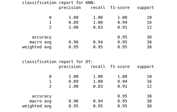
The scikit learn module also helps us calculate the precision, accuracy, f-score, and recall:

# Importing classification report
from sklearn.metrics import classification_report
# printing
print("classification report for KNN:\n", classification_report(y_test, KNN_predictions))
print("\nclassification report for DT:\n", classification_report(y_test, DT_predictions))

Output:

Evaluation of regression models

Different methods are available in the scikit learn module to evaluate the regression model. We will evaluate the Decision Tree and Random Forest regression models created in the above sections.

First, let’s find the mean absolute error using the scikit learn module:

# Importing mean_absolute_error from sklearn module
from sklearn.metrics import mean_absolute_error
# printing the mean absolute error
print("Means absolute error of Decision Tree is :",mean_absolute_error(y_test, DTR_predictions))
print("Means absolute error of Random forest is :",mean_absolute_error(y_test, RFR_predictions))

Output:

Other regressions evaluating metrics available in the scikit learn module are Mean Square Error (MSE) and Root Mean Square Error (RMSE).

Let’s apply these matrices to our model as well:

# Importing mean_squared_error from sklearn module
from sklearn.metrics import mean_squared_error
import math
# printing the mean squared error
print("Mean square error of Decision tree is :",mean_squared_error(y_test, DTR_predictions))
print("Mean square error of Random forest  is :",mean_squared_error(y_test, RFR_predictions))
print("\nRoot Mean square error of Decision tree is :",math.sqrt(mean_squared_error(y_test, DTR_predictions)))
print("Root Mean square error of Random forest  is :",math.sqrt(mean_squared_error(y_test, RFR_predictions)))

Output:

Models cross-validation

Cross-validation is a technique for evaluating ML models by training several ML models on subsets of the available input data and evaluating them on the complementary subset of the data. It can be handy in detecting the overfitting of the model.

Computing cross-validation in scikit learn

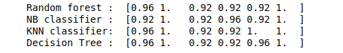
The simplest way to use cross-validation is to use cross_val_score from the scikit learn module. In the following example, we will see how to estimate the accuracy of various models by fitting the models and computing the score 6 consecutive times:

# importing the cross validation from sklearn
from sklearn.model_selection import cross_val_score
from sklearn import datasets
# loading the iris dataset
Input, Target = datasets.load_iris(return_X_y=True)

# initializing the models 
RF_classifier = RandomForestClassifier(n_estimators = 50)
NB_classifier = GaussianNB()
KNN_classifer = KNeighborsClassifier(n_neighbors=5)
DT_classifier = tree.DecisionTreeClassifier()

# calculating the scores for each model using cross validation
score1 = cross_val_score(RF_classifier, Input, Target, cv=6)
score2 = cross_val_score(NB_classifier, Input, Target, cv=6)
score3 = cross_val_score(KNN_classifer, Input, Target, cv=6)
score4 = cross_val_score(DT_classifier, Input, Target, cv=6)

# printing
print("Random forest : ", score1)
print("NB classifier : ", score2)
print("KNN classifier: ", score3)
print("Decision Tree : ", score4)

Output:

The cross_val_score uses the KFold split strategy by default. We can change the cross-validation strategies by passing a cross-validation iterator. For example, see the example below:

# importing the module
from sklearn.model_selection import ShuffleSplit
    
# creating iterator
cv = ShuffleSplit(n_splits=6, test_size=0.3, random_state=0)

# calculating the scores for each model using cross validation
score1 = cross_val_score(RF_classifier, Input, Target, cv=cv)
score2 = cross_val_score(NB_classifier, Input, Target, cv=cv)
score3 = cross_val_score(KNN_classifer, Input, Target, cv=cv)
score4 = cross_val_score(DT_classifier, Input, Target, cv=cv)
# printing
print("Random forest : ", score1)
print("NB classifier : ", score2)
print("KNN classifier: ", score3)
print("Decision Tree : ", score4)

Output:

Cross-validation iterators

We assume that the data is independent and identically distributed when using cross-validation iteration. Downbelow, we will apply various cross-validation methods to iterate data and split it into the training and testing parts.

Let’s say we have the following dataset.

# importing the module
import numpy as np
# creating dataset
data = np.array([[1, 2], [3, 4], [5, 6], [7, 8],[9,10],[9,4],[6,3],[2,1],[0,9]])
# printing
print(data)

Output:

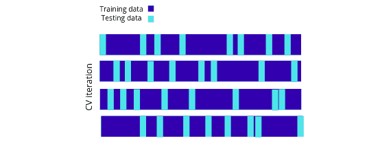
K-fold

K-fold divides all the samples into groups of k samples known as folds. The following is the pictorial representation of K-fold cross-validation.

Let’s use the scikit learn module to implement the K-fold cross-validation on the dataset:

# Importing the kfold module
from sklearn.model_selection import KFold
# initializing the k-fold 
k_fold = KFold(n_splits=6)
# iterating over dataset
for train, test in kf.split(data):
    print("Training: %s, Testing: %s" % (train, test))

Output:

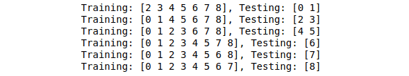
Notice that each time it is assigning different data for the testing part.

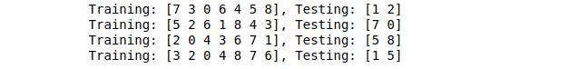
Shuffle split iterator

The ShuffleSplit iterator will generate a user-defined number of independent train/test dataset splits. Samples are first shuffled and then split into a pair of train and test sets:

Let’s use the ShuffleSplit iterator using the scikit learn module on the dataset:

# Importing shuffle split iterator
from sklearn.model_selection import ShuffleSplit
# initializing shuffle split iterator
shuffle_split = ShuffleSplit(n_splits=4, test_size = 0.2)
# iterating over dataset
for train, test in ss.split(data):
    print("Training: %s, Testing: %s" % (train, test))

Output:

Summary

Scikit-learn is the most useful Machine Learning Python library in Computer Science. This article covered the scikit learn library, which contains many efficient tools, ML, and statistical algorithms, including classification, regression, clustering, and many others.