Introduction to SciPy

SciPy is an open-source scientific computing library for Python that depends on NumPy. At a high level, NumPy offers you convenient and fast N-dimensional NumPy arrays manipulation, and the goal of SciPy is to give you additional user-friendly functionality for numerical integration, optimization, stats, and signal processing. This article will cover the basics of SciPy and its various submodules.

Installation of SciPy

The SciPy library consists of sub-packages covering different scientific computing domains. Here’s the list of the most commonly used ones:

• constants – contains physical and mathematical constants and units
• integrate – this package provides several integration techniques, including an ordinary differential equation integrator
• interpolate – this package contains spline functions and classes, 1-D, and univariate and multivariate multidimensional interpolation
• linalg – linear algebra functions
• ndimage – various functions for multidimensional image processing
• stats – this module contains a large number of probability distributions, summary and frequency statistics, correlation functions and statistical tests, masked statistics, kernel density estimation, quasi-Monte Carlo functionality, and more

Before reviewing the modules above, let’s install the SciPy library on our system. We can use the pip command to install the module by typing the following command:

pip install scipy

You can check the version of the installed SciPy module by using the following Python code:

# Importing the module
import scipy
# printing the version
print(scipy.__version__)

The installed version of the SciPy module on my system is 1.6.1

Constants in SciPy

The SciPy constants package (constants) provides a wide range of constants used in general scientific areas. To get access to constants, you need to import the module first:

# importing the constants
from scipy import constants

Mathematical constants

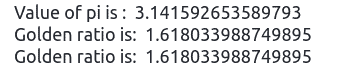
The mathematical constants include pi, golden and golden ratio, which we can import and print out as shown below:

# printing mathematical constants
print("Value of pi is : ", constants.pi)
print("Golden ratio is: ", constants.golden_ratio)
print("Golden ratio is: ", constants.golden)

Output:

Physical constants

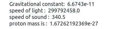
Physical constants include the speed of light, gravitational constant, gravitational acceleration, proton mass, neutron mass, and many more.

# printing Physical constants
print("Gravitational constant: ", constants.gravitational_constant)
print("speed of light : ", constants.speed_of_light)
print("speed of sound : ", constants.speed_of_sound)
print("proton mass is : ", constants.proton_mass)

Output:

Measurement units

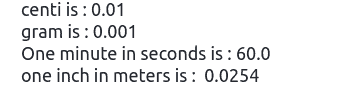
Finally, the constants module contains various measurement units:

# printing some units
print("centi is :", constants.centi)
print("gram is :", constants.gram)
print("One minute in seconds is :", constants.minute)
print("one inch in meters is : ", constants.inch)

Output:

Integration in SciPy

In mathematics, an integral assigns numbers to functions in a way that describes displacement, area, volume, and other concepts that arise by combining infinitesimal data. The process of finding integrals is called integration.

Wikipedia

The SciPy library provides an integral module (integrate) to calculate complex integrals without manual efforts. In the following sections of the article, we will use SciPy to calculate single and double integrals.

Single integral

The integration operation finds out the area under the curve of an arbitrary function.

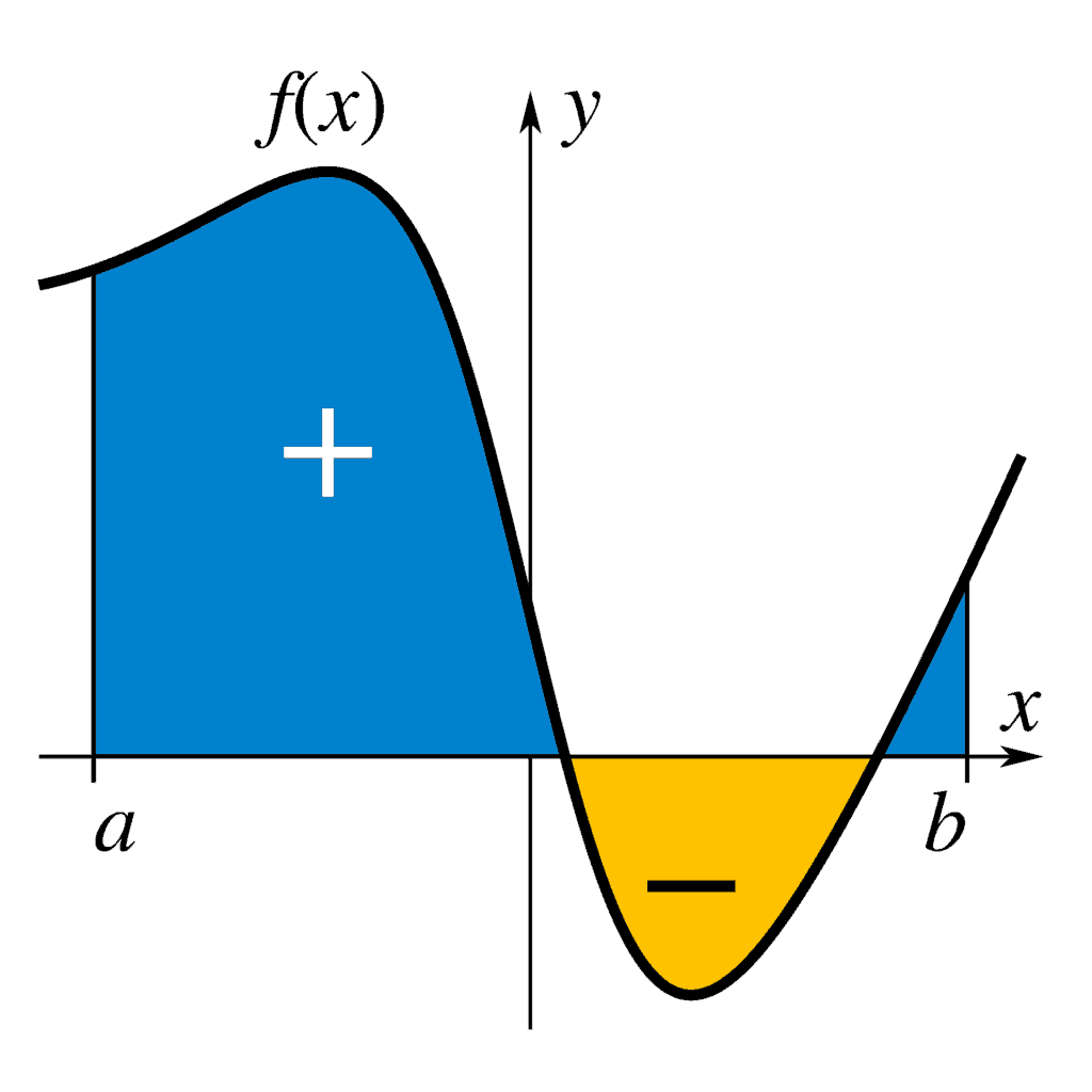
In SciPy, we can calculate the single integral by calling the quad() method:

scipy.integrate.quad(f, a, b)

The quad() method takes three arguments:

• f is the function
• a is the start of the interval
• b is the end of the interval

For example, we have the following function, and we want to calculate the integral using the SciPy library:

Let’s use SciPy to solve the above problem:

# importing required modules
from scipy import integrate
from numpy import exp
# defining function
function = lambda x:exp(-x**3)
# finding integral (function sum)
integral = scipy.integrate.quad(function, 0, 1)
# output
print(integral)

Output:

The quad() function returns the two values:

• the first number is the value of the integral
• the second value is the estimate of the absolute error in the value of the integral

Double integral

Double integrals are a way to integrate over a two-dimensional area, and they let us compute the volume under a surface.

In SciPy, we can calculate the double integral by calling the dblquad() method:

scipy.dblsquad(function, a, b, gfunc, hfunc)

The dblquad() method takes five arguments:

• function is the name of the function to be integrated
• a and b are the start and the end interval of the x variable
• gfunc and hfunc are names of functions that define the lower and upper intervals of the y variable

Let’s define some random functions and find the double integration using the SciPy library:

# importing the module
from math import sqrt
# defining the functions
function = lambda x, y : 8*x*y
gfunc = lambda x : 0
hfunc = lambda y : sqrt(1-3*y**3)
# finding double integral
integral = scipy.integrate.dblquad(function, 0, 0.5, gfunc, hfunc)
# printing
print(integral)

Output:

Similarly, you can also find triple integral and n-fold integral.

Interpolation in SciPy

The interpolation is the process of finding a value between two points on a line or a curve. Interpolation is useful in statistics and science, business, or when there is a need to predict values that fall within two existing data points.

Let’s create some datasets, and then we will apply interpolation:

# importing the required module
import numpy as np
# creating two datasets
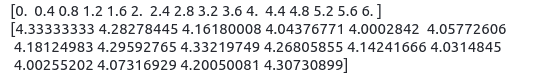
x_axis = np.linspace(0, 6, 16)
y_axis = np.cos(x_axis)**2/3+4
# printing
print(x_axis)
print(y_axis)

Output:

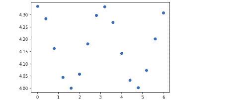
We will now visualize the dataset to see it more clearly using matplotlib module:

# Importing the module
import matplotlib.pyplot as plt

# ploting the dataset
plt.plot(x_axis, y_axis, 'o')
plt.show()

Output:

1-D interpolation

The interp1d class in the scipy.interpolate module is a convenient method to create a function based on fixed data points, which can be evaluated within the domain defined by the given data using linear interpolation. In mathematics, linear interpolation is a method of curve fitting using linear polynomials to construct new data points within the range of a discrete set of known data points.

Let’s use the above data points to create a interpolate function and draw a new interpolated graph:

# importing the module
from scipy import interpolate
# creating functions
func1 = interpolate.interp1d(x_axis, y_axis, kind = 'linear')
func2 = interpolate.interp1d(x_axis, y_axis, kind = 'cubic')

We’ve created two functions using the interp1d class, which takes any input for the x and y axes, and the kind of the interpolation type (Nearest, Zero, Linear, Quadratic, or Cubic).

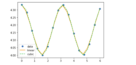
Let’s visualize these functions on a graph:

# Creating new input length
x_new = np.linspace(0, 6,20)
# Ploting the graph
plt.plot(x_axis, y_axis, 'o', x_new, func1(x_new), '-', x_new, func2(x_new), '--')
plt.legend(['data', 'linear', 'cubic','nearest'], loc = 'best')
plt.show()

Output:

Spline curve

A spline curve is a special function defined piecewise by polynomials that allow easily building of an interface for a user to design and control the shape of complex curves and surfaces. The general approach is that the user enters a sequence of points, and a machine constructs a curve that closely follows the series of defined points. Defined points are called control points. A curve that passes through each control point is called an interpolating curve, and a curve that follows near the control points but not necessarily through them is called an approximating curve.

We will use the UnivariateSpline class from the SciPy module, a 1-D smoothing spline that fits a given group of data points.

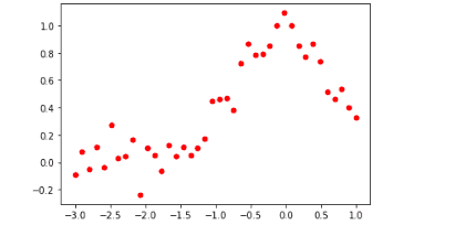
Let’s create some data points and visualize them:

# creating new data points
x_axis = np.linspace(-3, 1, 50)
y_axis = np.exp(-x_axis**2) + 0.1 * np.random.randn(50)
# ploting the graph
plt.plot(x_axis, y_axis, 'ro', ms = 5)
plt.show()

Output:

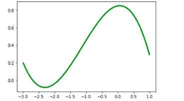
Now, we can produce a line that fits the above points:

# importing the module
from scipy.interpolate import UnivariateSpline
# initializing the univariate spline
U_p = UnivariateSpline(x_axis, y_axis)
xs = np.linspace(-3, 1, 100)
# ploting
plt.plot(xs, U_p(xs), 'g', lw = 3)
plt.show()

Output:

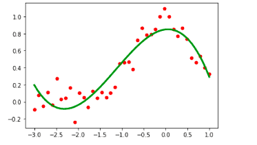
Let’s plot both graphs appended to see the difference:

plt.plot(x_axis, y_axis, 'ro', ms = 5)
plt.plot(xs, U_p(xs), 'g', lw = 3)
plt.show()

Output:

Linear algebra in SciPy

Linear Algebra is a branch of mathematics concerned with mathematical structures closed under the operations of addition and scalar multiplication. That includes the theory of systems of linear equations, matrices, determinants, vector spaces, and linear transformations.

You can use the linalg module to solve linear algebraic expressions.

Linear Equations

A linear equation between two variables gives a straight line when plotted on a graph. The scipy.linalg.solve feature solves the linear equation a * x + b * y = Z for the unknown x and y values.

Let’s say we have the following linear equations:

Let’s define these functions using NumPy and then solve this equation system:

# Importing therequired modules
import numpy as np
from scipy import linalg
# creating the function with inputs and outputes
Inputs = np.array([[4, 3, -5],
             [-2, -4, 5], 
              [8, 8, 0]])
Outputs = np.array([2, 5, -3])
# solving the equation 
solution = scipy.linalg.solve(Inputs, Outputs)
# printing solution
print(solution)

Output:

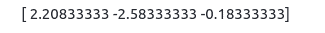
These are the values of x, y, and z, respectively.

Determinants

The determinant is a scalar value that is a function of the entries of a square matrix. It allows characterizing some properties of the matrix and the linear map represented by the matrix. The determinant of a matrix, let’s say A is often denoted as |A|.

In SciPy, the determinant is computed using the det() function. It takes a matrix as input and returns a scalar value.

Let’s create a square matrix and then apply the det() function to calculate its determinant:

#importing the scipy 
from scipy import linalg
#Declaring the numpy array
matrix = np.array([[4,5, 2],[4, 5, 6],[7, 8, 9]])
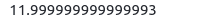
#Passing the values to the det function
determinant = linalg.det(matrix)
#printing
print(determinant)

Output:

Eigenvalues and eigenvectors

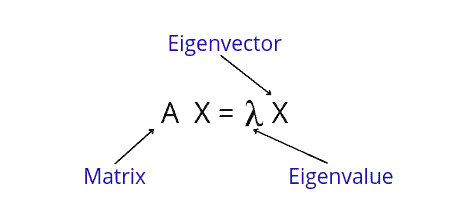
Let A be an n × n matrix and let X be a nonzero vector for which the following equation is true:

AX=λX

For some scalar λ, an eigenvalue of the matrix A and X is called an eigenvector of A associated with λ.

The scipy.linalg.eig() function computes the eigenvalues from a common or generalized eigenvalue problem. This function returns the eigenvalues and the eigenvectors.

Let’s take a simple example and find eigenvalues and eigenvectors:

#importing the scipy and numpy packages
from scipy import linalg
import numpy as np
#Declaring the numpy array
Matrix = np.array([[1,2, 3],[9, 8, 7], [6, 5, 4]])
#Passing the values to the eig function
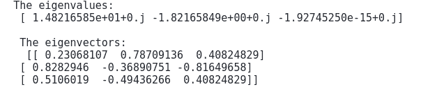
eigen_value, eige_vector = linalg.eig(Matrix)
#printing the result for eigen values and eigenvectors
print ("The eigenvalues: \n", eigen_value)
print ("\n The eigenvectors:\n ", eige_vector)

Output:

Singular Value Decomposition

A Singular Value Decomposition can be thought of as an extension of the eigenvalue problem to matrices that are not square. The scipy.linalg.svd() function factorizes the matrix into two unitary matrices in such a way that:

Matrix = U*S*Vh

Here, the S is a suitably shaped matrix of zeros with the main diagonals.

Let’s take an example and solve using the SciPy module:

#Declaring the numpy array
Matrix = np.array([[1,2, 3],[9, 8, 7], [6, 5, 4]])
#Passing the values to the eig function
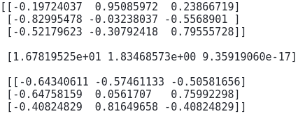
U, s, Vh = linalg.svd(Matrix)
# printing the result
print(U)
print("\n",s)
print("\n",Vh)

Output:

Statistic and SciPy

Statistics is the science of developing and studying methods for collecting, analyzing, interpreting, and presenting empirical data. Machine learning and statistics are two tightly related fields of study. Statistics is considered a prerequisite subject for machine learning as machine learning developers need statistics to transform observations into information and answer questions about observations’ samples.

The scipy.stats module contains all the statistics functions in SciPy. In this section, we will explore some of the statistics functions of this module.

Normal Distribution

Normal Distribution (or Gaussian Distribution) is a probability function that describes how the values of a variable are distributed.

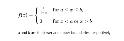
The probability density function of the normal distribution is defined as:

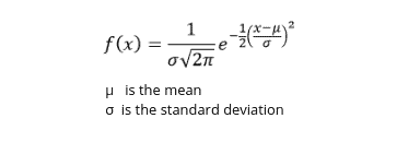
The probability density function scipy.stats.pdf can take up to three parameters:

scipy.stats.norm.pdf(x, loc=0, scale=1)

Here, the x is a required variable representing the random variable, while the other two are optional parameters representing the distribution’s mean and standard deviation.

The probability distribution function of normal distribution

The norm.pdf() method represents the probability distribution function and is used to create normal distribution in SciPy.

Let’s create a normal distribution using this method:

# Importing the module
from scipy.stats import norm
#creating an array of values between -10 to 10 with a difference of 0.5
array = np.arange(-10, 10, 0.5)
# creating distribution
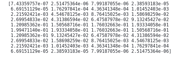
distribution = norm.pdf(array, 0, 2)
# printing the distribution
print(distribution)

Output:

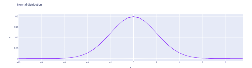
Now, we can visualize the above distribution:

# importing the module
import plotly.express as px
# ploting the distribution
fig = px.line(x=array, y=distribution, title='Normal distribution')
fig.show()

Output:

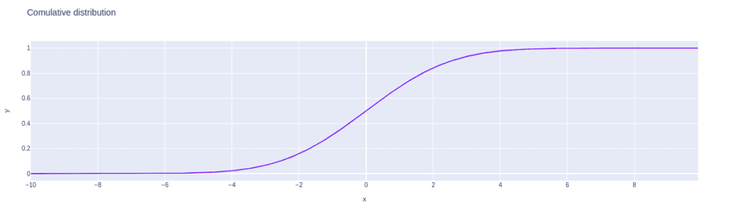
The cumulative distribution function of normal distribution

 The norm.cdf() function returns the cumulative distribution function of the distribution.

Let’s apply this method to calculate the cumulative distribution of the normal distribution:

#creating an array
array = np.arange(-10, 10, 0.1)
   
# creating commulative distribution 
distribution = norm.cdf(array, 0, 2)

Now can visualize the cumulative distribution that we have created above:

# ploting the comulative distribution
fig = px.line(x=array, y=distribution, title='Comulative distribution')
fig.show()

Output:

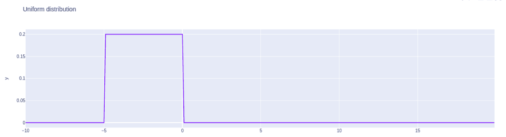
Unifrom distribution

A uniform distribution (or rectangular distribution) is a distribution where all values have equal probability between the distribution minimum and maximum.

The following formula is used for the probability density function of uniform distribution:

Uniform distribution describes an experiment where a random outcome that lies within certain bounds. The bounds of the outcome are defined by parameters a and b, which are the minimum and maximum values.

The probability distribution function of uniform distribution

The uniform.pdf() function measures the probability density function of the uniform distribution.

Let’s create a uniform distribution and visualize the probability density function:

# importing the required module
from scipy.stats import uniform
#creating an array of values between -5 to 10 with a difference of 0.5
array = np.arange(-10, 20, 0.1)
# creating a uniform distribution
U_distribution = uniform.pdf(array, -10, 5)

This will return a uniform distribution between -5 to 5. Let us now visualize the distribution by using the Plotly module.

# plotting the distribution
fig = px.line(x=array, y=U_distribution, title='Uniform distribution')
fig.show()

Output:

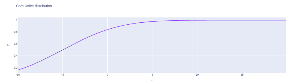
The cumulative distribution function of the uniform distribution

The uniform.cdf() method calculates the cumulative distribution of the uniform distribution.

Let’s calculate the cumulative distribution of our uniform distribution:

#creating an array
array = np.arange(-10, 20, 0.1)
# creating commulative distribution 
U_distribution = norm.cdf(array, -5, 5)

Now we can visualize the cumulative distribution using the Plotly module:

# plotting the distribution
fig = px.line(x=array, y=U_distribution, title='comulative distribution')
fig.show()

Output:

Binomial distribution

The binomial distribution is a type of distribution that has two possible outcomes. You can imagine it as a simple probability of a SUCCESS or FAILURE outcome in an experiment or survey that is repeated multiple times.

The formula gives the probability mass function (pmf) of the binomial distribution:

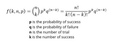
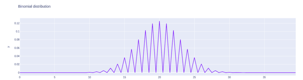
Probability mass distribution of binomial distribution

The binom.pmf() is used to calculate the probability mass distribution of the binomial distribution.

Let’s use this function to create a binomial mass distribution:

# importing the required module
from scipy.stats import binom
#creating an array of values between 0 to 40 with a difference of 0.5
array = np.arange(0, 40, 0.5)
   
# creating binomial distribution
B_distribution = binom.pmf(array, 40, 0.5)

Now we can visualize the binomial distribution:

# plotting the distribution
fig = px.line(x=array, y=B_distribution, title='Binomial distribution')
fig.show()

Output:

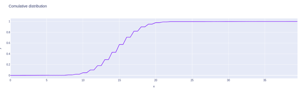
The cumulative distribution function of binomial distribution

The binom.cdf() method returns the distribution’s cumulative distribution function.

Let’s visualize the cumulative distribution of the binomial distribution:

#creating an array
array = np.arange(0, 40, 0.5)
# creating commulative distribution 
B_distribution = binom.cdf(array, 30, 0.5)
# plotting the distribution
fig = px.line(x=array, y=B_distribution, title='Cumulative distribution')
fig.show()

Output:

Geometric distribution

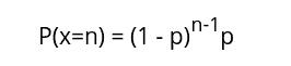
Geometric distribution can be defined as a discrete probability distribution representing the probability of getting the first success after having a consecutive number of failures. A geometric distribution can have an indefinite number of trials until the first success is obtained. In other words, it is a probability distribution of the random variable X representing the number of Bernoulli trials needed to get one success.

The geometric distribution gives the probability that the first occurrence of success requires n independent trials, each of which has the success probability of p. If the probability of the success on each trial is p, then the probability that the n-th trial (out of n trials) is the first success is given by the formula:

Let’s now find the probability mass distribution and visualize it.

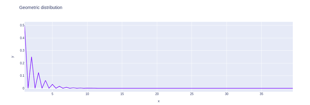
Probability mass function of geometric distribution

The geom.pmf() method measures the probability mass function of the geometric distribution.

Let’s use this method to find the mass distribution of geometric distribution:

# importing the module
from scipy.stats import geom
#creating an array of values between 1 to 40 with a difference of 0.5
array = np.arange(1, 40, 0.5)
   
# applying pmf function
G_distribution = geom.pmf(array, 0.5)

Now, we can visualize the geometric distribution:

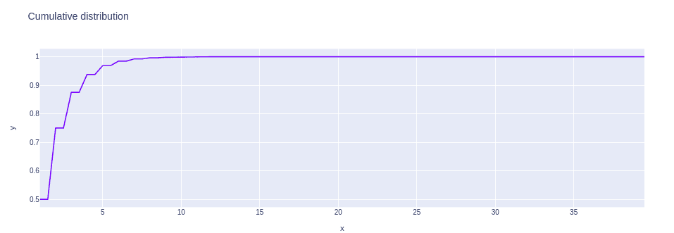
The cumulative distribution function of geometric distribution

The geom.cdf() method returns the cumulative distribution function of the geometric distribution.

Let’s find the cumulative distribution and then visualize it:

#creating an array of values between 1 to 40 with a difference of 0.5
array = np.arange(1, 40, 0.5)
# distribution 
G_distribution = geom.cdf(array, 0.5)
# plotting the distribution
fig = px.line(x=array, y=G_distribution, title='Cumulative distribution')
fig.show()

Output:

Descriptive statistics

Descriptive statistics is used to describe the basic features of the data. It provides simple summaries of the sample and the measures. Descriptive Statistics is used to present quantitative descriptions in a manageable form, for example, mean, mode, median, variance, etc.

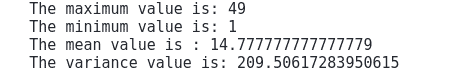
Let’s create a simple dataset and find the mean, minimum, maximum, and variance:

# importing the module
from scipy import stats
# creating the dataset
data = np.array([1,5,23,49,5,26,7,8,9])
# printing
print("The maximum value is:", data.max())
print("The minimum value is:", data.min())
print("The mean value is :", data.mean())
print("The variance value is:", data.var())

Output:

Processing images

The ndimage submodule in SciPy is used for image processing. Image processing is a method to perform some operations on an image to get an enhanced image or extract some useful information from it. Some of the most common tasks in image processing are opening images, cropping, flipping, rotating, filtering, classification, and many more. This section will apply some of these image processing methods to a sample image.

Opening image file in SciPy

The misc module in SciPy comes with some images. We can use those images to learn the image manipulation functions.

First, let’s open one of the images:

# Importing the module
from scipy import misc
# loading the image
img = misc.face()
# printing
print(img)

Output:

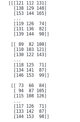
The output is in the form of a matrix. We can use matplotlib module to show the image:

# importing the module
import matplotlib.pyplot as plt
# showing the image
plt.imshow(img)
plt.show()

Output:

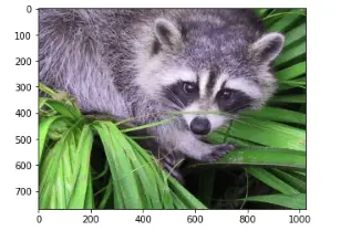
Image display attributes

We can display the image by changing its color, contrast level, brightness, and other properties.

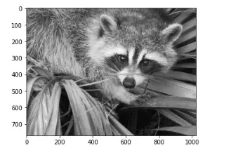
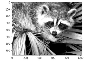
Let’s display the image in a grayscale form:

# retrieve a gray image
img = misc.face(gray=True)  
# plotting the image
plt.imshow(img, cmap=plt.cm.gray)        
plt.show()

Output:

To increase the contrast level of our image, we can set the vmin and vmax arguments:

# increase the contrast level
plt.imshow(img, cmap=plt.cm.gray, vmin=30, vmax=200)   
plt.show()

Output:

Cropping the image

The image variable stores an array of numbers representing the color of each image pixel. You can change these numbers to alter the original image.

Let’s perform a geometric transformation on the image and crop the image:

# finding the shape of the image
lx, ly = img.shape
# printing
print(lx, ly)

Output:

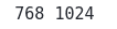
Now, we can change the shape of the image to crop it:

# cropping the image
crop_face = img[int(lx / 4): int(- lx / 4), int(ly / 4): int(- ly / 4)]
# finding the shape of the cropped image
lx, ly = crop_face.shape
# printing
print(lx, ly)

Output:

That’s how we’ve reduced the shape of our image.

Let’s now plot the result of our operation:

# plotting
plt.imshow(crop_face)
plt.show()

Output:

Rotating the image

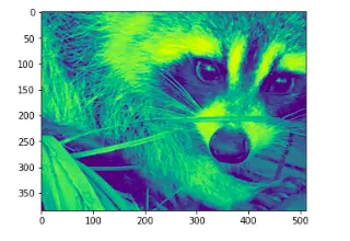
We can also rotate the image upside down by using NumPy’s flipud() method:

# importing the image
img = misc.face()
# flipping the image
flipping = np.flipud(img)
# plotting the image
plt.imshow(flipping)
plt.show()

Output:

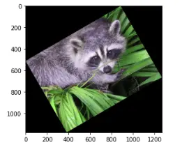
Moreover, by using rotate() method, we can rotate an image to a specified degree.

For example, let’s rotate the image by 30 degrees:

# importing the module
from scipy import ndimage
# rotating the image
rotated = ndimage.rotate(img, 30)
# plotting
plt.imshow(rotated)
plt.show()

Output:

You can learn more about the SciPy and image processing from the article Image manipulation and processing using Numpy and Scipy.

Summary

SciPy is an open-source scientific library for Python that depends on NumPy. The goal of SciPy is to give you additional user-friendly functionality for optimization, stats, and signal processing. In this article, we’ve covered the basics of SciPy and its various submodules.