In this article, we’ll give you the most commonly used tools for data preprocessing in machine learning, including:
Let’s create a hypothetical dataset for a small retail business that tracks sales data for different products across various stores. This dataset will include some categorical data, numerical data, and intentionally include some missing values to demonstrate data preprocessing techniques.
Dataset
- Store_ID: The unique identifier for each store (categorical).
- Product: The type of product sold (categorical).
- Units_Sold: The number of units sold (numerical).
- Revenue: The total revenue generated from the product at that store (numerical).
- Customer_Rating: Average customer rating for the product at the store (numerical).
Here’s a small sample dataset:
| Store_ID | Product | Units_Sold | Revenue | Customer_Rating |
|---|---|---|---|---|
| 001 | Toy | 53 | 795.0 | 4.3 |
| 002 | Book | NaN | 450.0 | 4.1 |
| 003 | Electronics | 34 | NaN | 3.9 |
| 004 | Toy | 24 | 360.0 | NaN |
| 001 | Book | 44 | 660.0 | 4.5 |
| 002 | Electronics | 21 | 315.0 | 4.0 |
| 003 | Toy | 29 | 435.0 | 4.2 |
| 004 | Book | NaN | 240.0 | 3.8 |
Dataset Import
The code below creates a DataFrame from a string. In a real scenario, you would likely load the data from a CSV file using pd.read_csv('path/to/your/file.csv'). This dataset includes some missing values (NaN) in Units_Sold, Revenue, and Customer_Rating columns, which can be addressed using the preprocessing steps outlined in the article.
import numpy as np
import pandas as pd
from io import StringIO
data = """
Store_ID,Product,Units_Sold,Revenue,Customer_Rating
001,Toy,53,795,4.3
002,Book,,450,4.1
003,Electronics,34,,3.9
004,Toy,24,360,
001,Book,44,660,4.5
002,Electronics,21,315,4.0
003,Toy,29,435,4.2
004,Book,,240,3.8
"""
# Using StringIO to simulate reading from a file
dataset = pd.read_csv(StringIO(data))
print(dataset.head())
Deleting unneeded information
In the context of data preprocessing for machine learning, one common step is the removal of unneeded information. This step is crucial because it helps in focusing on the relevant data, reducing the dimensionality, and improving the efficiency of machine learning models.
In the given dataset, we have several columns: Store_ID, Product, Units_Sold, Revenue, and Customer_Rating. If we determine that the Store_ID column is not relevant to our analysis or predictive modeling, we can remove it to simplify our dataset.
Here’s how we can remove the Store_ID column from the dataset:
# Dropping the 'Store_ID' column
dataset = dataset.drop(columns=['Store_ID'])
print(dataset.head())
Dealing with missing data
Missing data can lead to biased models, incorrect conclusions, or runtime errors if not addressed properly. One common technique for dealing with missing data is imputation, where missing values are replaced with substituted values. The SimpleImputer class from sklearn.impute is a convenient tool for this task.
In our dataset, we have missing values in the Units_Sold and Revenue columns. We can apply SimpleImputer to replace these missing values with the mean of the respective columns. This approach assumes that the missing values are randomly distributed and that their replacements with the mean value will not introduce significant bias.
Here’s how you can use SimpleImputer with the mean strategy to handle missing data in the dataset:
from sklearn.impute import SimpleImputer
# Initialize the SimpleImputer with strategy as 'mean'
imputer = SimpleImputer(missing_values=np.nan, strategy='mean')
# We apply imputation only on numerical columns. In this case, 'Units_Sold', 'Revenue', and 'Customer_Rating'
numerical_columns = ['Units_Sold', 'Revenue', 'Customer_Rating']
dataset[numerical_columns] = imputer.fit_transform(dataset[numerical_columns])
# Displaying the first few rows of the dataset after imputation
print(dataset.head())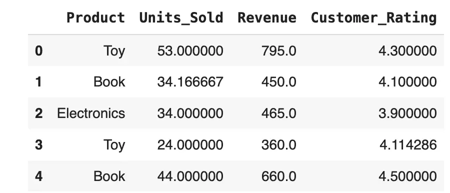
Encoding Categorical Data
Categorical data encoding is essential in data preprocessing for machine learning as most algorithms can only work with numerical data. Two common methods for encoding categorical variables are One-Hot Encoding and Label Encoding. One-Hot Encoding is used when the categorical variable is nominal (no intrinsic order), while Label Encoding is typically used for ordinal data (there is a natural order).
| Feature | One-Hot Encoding | Label Encoding |
|---|---|---|
| Description | Converts each unique category value into a new binary column (0 or 1). | Converts each category value into a unique integer. |
| Use Case | Ideal for nominal data where no ordinal relationship exists between categories. Examples include colors, city names, or product types. | Suitable for ordinal data where the categories have an intrinsic order or hierarchy, like ‘low’, ‘medium’, ‘high’, or ‘yes’ and ‘no’. |
| Number of Columns | Creates additional columns equal to the number of unique category values. For a column with n categories, n new columns will be created. | Keeps the number of columns the same, replacing the original column with the integer-encoded one. |
| Model Impact | Prevents the model from assuming an order or importance where none exists, but increases the dimensionality of the dataset (potential issue with high cardinality). | Implies an order or importance which might not exist in the data, potentially leading to model misinterpretation if used on nominal data. |
| Scalability | Can lead to a large increase in dataset size with high-cardinality categorical features, which may affect model performance and require more computational power. | Efficient in terms of space, as it maintains the dataset size, but may introduce ordinality where it is not appropriate, affecting model interpretation. |
| Example | Converting the Product column into three separate columns: Product_Toy, Product_Book, Product_Electronics, with binary values. | Converting Product types into integers like 0 for Toy, 1 for Book, and 2 for Electronics, etc. |
When to use which:
- Use One-Hot Encoding when the categorical variable is nominal (no order) to ensure that the model does not attribute a hierarchy where there isn’t one.
- Use Label Encoding for ordinal data where the categories have an intrinsic order or hierarchy that might be relevant to the predictive model.
One-Hot Encoding
One-Hot Encoding is used to convert categorical data into a format that can be provided to ML algorithms to do a better job in prediction. It converts each category value into a new column and assigns a 1 or 0 (notation for true/false).
Here’s how to apply One-Hot Encoding using ColumnTransformer and OneHotEncoder:
from sklearn.compose import ColumnTransformer
from sklearn.preprocessing import OneHotEncoder
# Applying One-Hot Encoding to the 'Product' column
ct = ColumnTransformer(transformers=[('encoder', OneHotEncoder(), ['Product'])], remainder='passthrough')
dataset_encoded = ct.fit_transform(dataset)
# Converting the array back to a dataframe
dataset_encoded = pd.DataFrame(dataset_encoded, columns=ct.get_feature_names_out())
print(dataset_encoded.head())
Label Encoding
Label Encoding converts each category into a unique integer based on alphabetical ordering. It is suitable for ordinal data where the order matters.
Here’s how to apply Label Encoding using LabelEncoder:
from sklearn.preprocessing import LabelEncoder
# Reusing the 'dataset' from the previous example
le = LabelEncoder()
# Applying Label Encoder to the 'Product' column
dataset['Product_encoded'] = le.fit_transform(dataset['Product'])
print(dataset.head())
In this code snippet, LabelEncoder assigns a unique integer to each category of the Product column. The transformed data shows the original and encoded values side by side for comparison.

Feature Selection and Target Setting
Feature selection is a critical process in machine learning where you identify the input variables (features) that are most relevant to the task of predicting the output variable (target). Proper feature selection improves model accuracy, reduces overfitting, and decreases computation time.
In our dataset, let’s consider Units_Sold as the target variable we want to predict, and the rest of the columns, except for Store_ID, as features.
Here’s how you can select features and target from the dataset:
# Feature selection: Dropping 'Revenue' (target)
features = dataset_encoded.drop(columns=['remainder__Revenue'])
# Target selection: Selecting 'Revenue' as the target
target = dataset_encoded['remainder__Revenue']
# Displaying the first few rows of features and target for illustration
print("Features:")
print(features.head())
print("\nTarget:")
print(target.head())
In this example:
- The features include encoded
Product,Revenue, andCustomer_Rating. - The target is
Revenue, which we aim to predict.
By isolating the features and target, we can now train machine learning models where the features are used to predict the target. This separation is fundamental in supervised learning to establish the relationship between input variables (features) and the output variable (target).
Splitting Data into Training and Testing Sets
Splitting your dataset into training and testing sets is a fundamental step in preparing your data for machine learning. The training set is used to train the model, while the testing set is used to evaluate its performance. This split is crucial for assessing the model’s ability to generalize to unseen data, helping prevent issues like overfitting.
Note: Always split the dataset before applying the feature scaling operation because you don’t want to introduce information leakage. The test set must always be unknown to the training algorithm.
Here’s how you can split your data into training and testing sets using the train_test_split function from sklearn.model_selection:
from sklearn.model_selection import train_test_split
# Splitting the dataset into 80% training and 20% testing
X_train, X_test, y_train, y_test = train_test_split(features, target, test_size=0.2)
# Displaying the sizes of the splits
print(f"Training features size: {X_train.shape}")
print(f"Testing features size: {X_test.shape}")
print(f"Training target size: {y_train.shape}")
print(f"Testing target size: {y_test.shape}")
Feature Scaling Using StandardScaler
Feature scaling is a crucial step in data preprocessing, especially for algorithms that compute distances or assume normality. Standardizing features by removing the mean and scaling to unit variance is a common approach. This is where StandardScaler from sklearn.preprocessing comes in handy.
| Standardisation | Normalisation |
|---|---|
| \(x’ = \frac{x-\mu(x)}{\sigma(x)}\) | \(x’ = \frac{x – \text{min}(x)}{\text{max}(x) – \text{min}(x)}\) |
| \(x’\) – is the standardized value of \(x\) \(x\) is the original value of the feature \(\mu(x)\) represents the mean of \(x\) \(\sigma(x)\) denotes the standard deviation of \(x\) | \(x’\) – is the standardized value of \(x\) \(x\) is the original value of the feature \(\text{min}(x)\) is the minimum value of the feature in the dataset \(\text{max}(x)\) is the maximum value of the feature in the dataset |
| This transformation converts all the features’ values between \([-3, 3]\) | This transformation converts all the features’ values between \([0, 1]\) |
| Safe to use it all the time | Works well only when you have normal distribution across most of your features |
StandardScaler standardizes features by subtracting the mean and scaling to unit variance. This standardization ensures that each feature contributes equally to the distance computations in algorithms like k-NN and k-means clustering, and it helps in speeding up the convergence of gradient descent-based algorithms.
Note: you don’t need to apply feature scaling to columns modified by the ColumnTransformer. Apply feature scaling only to columns initially stored numerical values.
Here’s how to apply StandardScaler to your features:
from sklearn.preprocessing import StandardScaler
# Initialize the StandardScaler
scaler = StandardScaler()
# Fit the scaler to the features and transform them
features_scaled = scaler.fit_transform(features)
# Converting the scaled features back to a DataFrame for better readability (optional)
features_scaled_df = pd.DataFrame(features_scaled, columns=features.columns)
# Displaying the first few rows of the scaled features
print(features_scaled_df.head())
In this code:
StandardScaleris initialized and then fitted to thefeaturesdata, which computes the mean and standard deviation to be used for later scaling.fit_transformmethod is applied tofeatures, which standardizes the features based on the computed mean and standard deviation.- The result is a set of features that are scaled to have zero mean and a variance of one, ensuring that all features are on a comparable scale.

This scaling is particularly beneficial for machine learning algorithms sensitive to the magnitude of features and helps in achieving better performance and faster convergence.
