Decision Tree Python – Easy Tutorial

A Decision Tree algorithm is a supervised learning algorithm for classification and regression tasks. It can be used to predict the outcome of a given situation based on certain input parameters. The algorithm creates a model of decisions based on given data, which can then be applied to unseen data to make predictions. As such, it is a useful tool for both classification and prediction tasks.

This Decision Tree Python tutorial covers the algorithm theory, implementation, performance evaluation, and dataset visualization. Let’s get started!

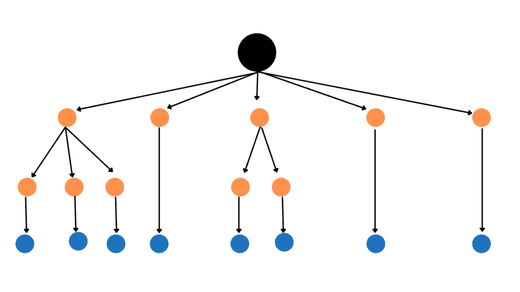
The Decision Tree can solve classification and regression problems, but it is most commonly used to solve classification problems. It is a tree-structured classifier, where internal nodes represent the features of a dataset, branches represent the decision rules, and each leaf node represents the decision outcome. The algorithm is called a Decision Tree because, like a tree, it starts with a root node that grows into more branches and forms a tree-like decision structure.

Using a Decision Tree algorithm allows us to mimic a human decision-making process when humans are making a choice. A tree-like structure allows us to simply and easily understand a decision-making process.

Terms and terminology

As the name suggests, the algorithm uses a tree-like decision-making structure in which each internal node represents a test on an attribute, each branch represents a test outcome, and each leaf node (terminal node) stores a class label. Here are some of the most important terminologies related to a Decision Tree:

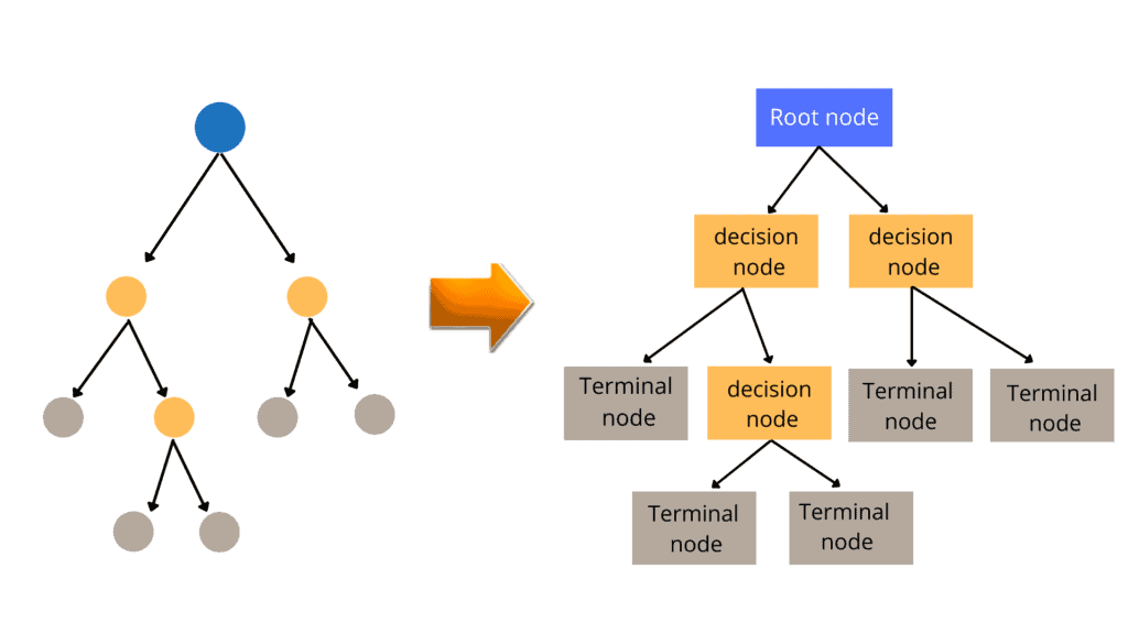
• Root Node: generally represents the entire sample and gets divided into two or more homogeneous sets. It is the very top node of the decision tree
• Splitting:  is a process of dividing a node into two or more sub-nodes
• Decision Node: a node or sub-node that splits data into further sub-nodes
• Leave Node: nodes that do not split is called Leaf or Terminal node; these are the final outputs of the decision tree
• Pruning: the opposite of splitting. When a sub-nodes of a decision node is removed, the process is called pruning
• Sub-Tree: a subsection of the entire tree is called a branch or sub-tree
• Parent Node:  a node, which is divided into sub-nodes, is called a parent node
• Child Node: any sub-nodes of a parent node are called Child Node

Let’s make the following assumptions while creating a Decision Tree:

• The entire dataset is considered a Root Node at the beginning
• Categorical feature values are preferred while making a Decision Tree. If the values are continuous, they must be discretized before the model can be built
• Records are distributed recursively based on attribute values
• Order to place attributes as root or internal nodes of the tree is done using some statistical approach. It is not randomly selecting one attribute as a root or internal node

How does a Decision Tree work?

The decision tree algorithm starts from the tree’s root node for predicting the class of the given dataset. It compares the values of the root attribute with the record/dataset attribute and, based on the comparison, follows the branch and jumps to the next node. Then the algorithm compares the attribute value with the other sub-nodes and moves on to the next node. It repeats the process until it reaches the tree’s leaf node. We can summarize the complete process of the decision tree in the following simple steps.

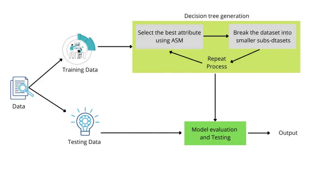
• Let’s say X is the root node that represents the entire dataset. The algorithm will start searching from the root node.
• The algorithm will find the best attribute in the dataset using any of the Attribute Selection Measure methods.
• The next step is to divide the root node X into subsets that contain possible values for the best attributes.
• Once the subsets are ready, it will generate the decision tree node containing the best attribute.
• Recursively create new decision trees using the subsets of the dataset created in the previous step. This step will continue until the nodes can no longer be classified, at that point, the final node is referred to as a leaf node.

Let’s consider the following example: an applicant received a job offer and is unsure whether to accept or reject it. The following decision tree helps him to decide:

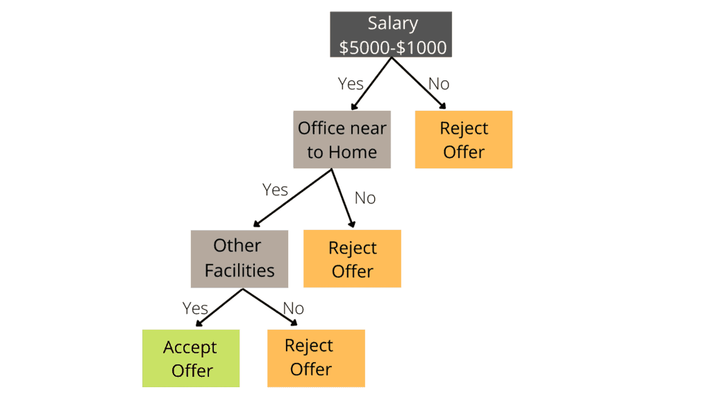
The decision tree above shows a candidate has been offered a job and is deciding whether to reject or accept the offer. The decision tree begins with the root node to address this problem (Salary attribute by ASM). The root node separates into the next decision node (distance from the home) and a single leaf node based on the related labels. The decision node splits into two leaf nodes at the end of the process (Accept the offer and Reject the offer). One decision node (Facilities) and one leaf node are created from the following decision node.

Attribute Selection Measurements in Decision Tree

The biggest challenge while developing a Decision Tree is choosing the best attribute for the root node and sub-nodes. The algorithm needs to find the best attribute for the root node and sub-nodes. For that purpose, we can use different attribute selection measurements method. For example, the information gain method and the Gini index. But before discussing these methods, let’s discuss entropy first.

Entropy

The uncertainty in our dataset or measure of disorder is called entropy. Its value describes the degree of randomness of a particular node. Such a situation occurs when the margin of difference for a result is thin, and the model doesn’t have confidence in the accuracy of the prediction. The higher the entropy, the more randomness will be in the dataset. Low entropy is preferred when using a Decision Tree algorithm. The general formula of entropy is:

Let us take an example and say that we have classes: class1 and class2. Then the entropy will be given as:

Let’s say class1 and class2 have the same number of entries. If we choose randomly one entry, it will belong to either class1 or class2, with a 50% chance of belonging to each of them. The entropy will be high in such cases.

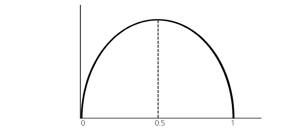
The probability of labeling varies with entropy, as shown in the diagram above. When the probability of a label is 0.5, the entropy is highest.

Information Gain

Information gain helps to determine the order of attributes in the nodes of a decision tree and decide whether a specific feature should be used to split a node.

Information gain is simply the measurement of entropy changes after a dataset’s segmentation based on an attribute. It calculates how much information a feature provides us about a class. We divide the nodes and build a decision tree based on the information gain value. The highest information gain node/attribute is split first in a decision tree method, which always maximizes the information gain value.

Gini Index

The Gini index, also known as the Gini impurity or Gini coefficient, measures the likelihood of a new instance of a random variable being incorrectly classified if it were randomly classified using the dataset’s distribution of class labels. Gini Index is also a measure of impurity used to build a decision tree. The lower the Gini score, the better.

 The Gini index is the summation of the square of the ratio of each class count in that node to the total instances in that node and then subtracted by 1.

Decision Tree Python Implementation

Let’s implement the Decision Tree algorithm using Python in AWS Sagemaker Studio and Jupyter Notebook. We will use some Python modules to implement the Decision Tree, which you can install on your Jupyter Notebook using the following commands in your cell.

% pip install sklearn
% pip install numpy
% pip install pandas
% pip install matplotlib

Once the modules are installed successfully, we can go to the implementation part. This section will use a sample dataset to train our model using a decision tree algorithm. You can access and download the sample dataset from this link.

Splitting dataset using the sklearn module

First, we must import all the necessary modules and the dataset we will use to train the model. Then we will split the dataset into input values and output values.

# importing the required modules
import matplotlib.pyplot as plt
import pandas as pd
# Importing the dataset using pandas module
dataset = pd.read_csv('decisionTree_Data.csv')
# splitting the dataset into input and output datasets
X = dataset.iloc[:, [0,1]].values
y = dataset.iloc[:, 2].values

The next step is to split the dataset into training data sets and testing datasets to check the accuracy of our model. We will use sklearn module for the splitting purposes of the dataset.

# splitting the dataaset into Training and Testing Data 
from sklearn.model_selection import train_test_split
# random state is 0 and test size if 25%
X_train, X_test, y_train, y_test = train_test_split(X,y,test_size=0.25, random_state=0)

We have assigned 75% of the original data to the training and 25% to the testing parts.

Training and Testing Decision Tree Algorithm

Once we split the data, the next step is to scale our dataset so the extreme values will not have too much effect on the prediction of our model.

# importing standard scalling method from sklearn
from sklearn.preprocessing import StandardScaler
sc = StandardScaler()
# providing the inputs for the scalling purpose
X_train = sc.fit_transform(X_train)
X_test = sc.transform(X_test)

Notice that we are only scaling the input values, not the output ones. Now, our data is ready for training the model using a decision tree algorithm.

# importing decision tree algorithm
from sklearn.tree import DecisionTreeClassifier
# entropy means information gain
classifer = DecisionTreeClassifier(criterion='entropy', random_state=0)
# providing the training dataset
classifer.fit(X_train,y_train)

Notice that we have imported the Decision Tree Python sklearn module class. We then used the information gain method to build a tree from the dataset. Finally, we provided both the inputs and outputs of the training data set to train our model.

Once the training is complete, we can provide the testing data to test our model. This time we will not provide the outputs. Instead, we will provide only the inputs, and the model will predict the outputs based on the training dataset.

y_pred = classifer.predict(X_test)

Let us test the accuracy of our model by importing the accuracy score method.

# importing the accuracy score
from sklearn.metrics import accuracy_score
# accuracy
accuracy_score(y_pred,y_test)

Output:

The accuracy of our model is 91%, which means our model classifies the test data 91% accurately.

Visualizing Decision Tree using Sklearn module in AWS Jupyter Notebook

We can also visualize the decision to see the results more accurately. There are many different ways to visualize a decision tree. Here we will use sklearn module to visualize our model.

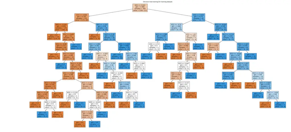
First, let us visualize the decision tree formed from our training dataset.

# importing the plot tree method
from sklearn.tree import DecisionTreeClassifier, plot_tree
clf = DecisionTreeClassifier()
# output size of decision tree
plt.figure(figsize=(40,20))
# providing the training dataset
clf = clf.fit(X_train, y_train)
plot_tree(clf, filled=True)
plt.title("Decision tree training for training dataset")
plt.show()

Output:

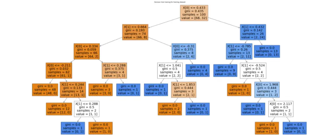
Similarly, we can also visualize the Decision Tree formed by the testing dataset.

# importing the plot tree method
from sklearn.tree import DecisionTreeClassifier, plot_tree
clf = DecisionTreeClassifier()
# output size of decision tree
plt.figure(figsize=(40,20))
# providing the training dataset
clf = clf.fit(X_test, y_test)
plot_tree(clf, filled=True)
plt.title("Decision tree training for testing dataset")
plt.show()

Output:

Visualizing Decision tree through text representation

Another way of visualizing the tree is text representation using skearn module. See the following text-based tree diagram.

# importing the tree
from sklearn import tree
# text based tree
text_representation = tree.export_text(clf)
print(text_representation)

Output:

|--- feature_0 <= 0.43
|   |--- feature_1 <= 0.66
|   |   |--- feature_0 <= 0.33
|   |   |   |--- feature_0 <= -0.21
|   |   |   |   |--- class: 0
|   |   |   |--- feature_0 >  -0.21
|   |   |   |   |--- feature_1 <= 0.24
|   |   |   |   |   |--- class: 0
|   |   |   |   |--- feature_1 >  0.24
|   |   |   |   |   |--- feature_1 <= 0.29
|   |   |   |   |   |   |--- class: 1
|   |   |   |   |   |--- feature_1 >  0.29
|   |   |   |   |   |   |--- class: 0
|   |   |--- feature_0 >  0.33
|   |   |   |--- feature_1 <= 0.29
|   |   |   |   |--- class: 0
|   |   |   |--- feature_1 >  0.29
|   |   |   |   |--- class: 1
|   |--- feature_1 >  0.66
|   |   |--- feature_0 <= -0.31
|   |   |   |--- feature_1 <= 1.04
|   |   |   |   |--- class: 1
|   |   |   |--- feature_1 >  1.04
|   |   |   |   |--- feature_1 <= 1.85
|   |   |   |   |   |--- class: 0
|   |   |   |   |--- feature_1 >  1.85
|   |   |   |   |   |--- class: 1
|   |   |--- feature_0 >  -0.31
|   |   |   |--- class: 1
|--- feature_0 >  0.43
|   |--- feature_1 <= 0.43
|   |   |--- feature_1 <= -0.79
|   |   |   |--- class: 1
|   |   |--- feature_1 >  -0.79
|   |   |   |--- feature_1 <= -0.52
|   |   |   |   |--- class: 0
|   |   |   |--- feature_1 >  -0.52
|   |   |   |   |--- feature_0 <= 1.97
|   |   |   |   |   |--- class: 1
|   |   |   |   |--- feature_0 >  1.97
|   |   |   |   |   |--- feature_0 <= 2.12
|   |   |   |   |   |   |--- class: 0
|   |   |   |   |   |--- feature_0 >  2.12
|   |   |   |   |   |   |--- class: 1
|   |--- feature_1 >  0.43
|   |   |--- class: 1

Decision Tree using Sklearn and AWS SageMaker Studio

Now let us implement the decision code using the sklearn module in AWS SageMaker Studio, using Python version 3.7.10.

First, let’s import the required modules and split the data, then train the data and test the model. This time we will show the result of the predictions using a confusion matrix.

# importing the required modules
import matplotlib.pyplot as plt
import pandas as pd
import seaborn as sns
# Importing the dataset using pandas module
dataset = pd.read_csv('decisionTree_Data.csv')
# splitting the dataset into input and output datasets
X = dataset.iloc[:, [0,1]].values
y = dataset.iloc[:, 2].values
# splitting the dataaset into Training and Testing Data 
from sklearn.model_selection import train_test_split
# random state is 0 and test size if 25%
X_train, X_test, y_train, y_test =train_test_split(X,y,test_size=0.25, random_state=0)
# importing standard scalling method from sklearn
from sklearn.preprocessing import StandardScaler
sc = StandardScaler()
# providing the inputs for the scalling purpose
X_train = sc.fit_transform(X_train)
X_test = sc.transform(X_test)
# importing decision tree algorithm
from sklearn.tree import DecisionTreeClassifier
# entropy means information gain
classifer=DecisionTreeClassifier(criterion='entropy', random_state=0)
# providing the training dataset
classifer.fit(X_train,y_train)
y_pred= classifer.predict(X_test)
# creating confusion matrix
from sklearn.metrics import confusion_matrix
cm = confusion_matrix(y_test,y_pred)
# Making the Confusion Matrix
cm = confusion_matrix(y_pred, y_test)
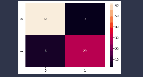
sns.heatmap(cm,annot=True)
plt.savefig('confusion.png')

Output:

Performance evalution of Decision Tree algroithm

Let us now understand how confident our model is in making predictions. One of the best ways to evaluate the model’s performance is by using a confusion matrix and other scoring functions. A confusion matrix is an error matrix table used for supervised classification tasks. Its functionality consists of plotting correct and incorrect predictions. In addition to this, you can use it for domain-specific metrics evaluations too. You can learn more about the confusion matrix from this article.

Evaluating Decision Tree for binary classification using a confusion matrix

The model we trained in the previous section was trained on a binary dataset because there were only two output classes. Let us now evaluate the model using a confusion matrix.

# importing the required modules
import matplotlib.pyplot as plt
from sklearn.metrics import confusion_matrix, ConfusionMatrixDisplay
# Plot the confusion matrix in graph
cm = confusion_matrix(y_test,y_pred, labels=classifer.classes_)
# ploting with labels
disp = ConfusionMatrixDisplay(confusion_matrix=cm, display_labels=classifer.classes_)
disp.plot()
# showing the matrix
plt.show()

Output:

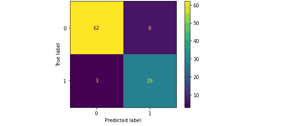
You can infer a lot of information from the confusion matrix above, which shows the results of the model’s predictions. Some of these are as follows:

• 62 out of 68 false classes were predicted accurately by the model, which means the accuracy for the prediction of the false class is 91%.
• 29 out of 32 True classes were predicted accurately by the model, which means the accuracy for the prediction of the True class is 90%.
• 9 out of 100 classes were classified incorrectly, meaning the overall percentage of classifying a class incorrectly is 9%.

Confusion Matrix Values

Print the True Positive, True Negative, False Positive, and False Negative values by using python code.

# defining a function which takes acutal and pred values
def confusion_values(y_actual, y_pred):
    # initializing the values with zero value
    TP = 0
    FP = 0
    TN = 0
    FN = 0
    # iterating through the values
    for i in range(len(y_pred)): 
        if y_actual[i]==y_pred[i]==1:
           TP += 1
        if y_pred[i]==1 and y_actual[i]!=y_pred[i]:
           FP += 1
        if y_actual[i]==y_pred[i]==0:
           TN += 1
        if y_pred[i]==0 and y_actual[i]!=y_pred[i]:
           FN += 1
    # printing the values
    print("True Positive: ", TP)
    print("False Positive:", FP)
    print("True Negative: ", TN)
    print("False Negative: ", FN)
# calling the function
confusion_values(y_test, y_pred)

Output:

• True Positive: A true positive is an outcome where the model correctly predicts the positive class.
• True Negative: A true negative is an outcome where the model correctly predicts the negative class.
• False Positive: A false negative is an outcome where the model incorrectly predicts the positive class.
• False Negative: A false negative is an outcome where the model incorrectly predicts the negative class.

Let us now determine the model’s accuracy, precision, recall, and f1-score using the confusion matrix.

# importing the required module and methods
from sklearn.metrics import accuracy_score, precision_score, recall_score, f1_score
print(f'Accuracy-score: {accuracy_score(y_test, y_pred):.3f}')
print(f'Precision-score: {precision_score(y_test, y_pred):.3f}')
print(f'Recall-score: {recall_score(y_test, y_pred):.3f}')
print(f'F1-score: {f1_score(y_test, y_pred):.3f}')

Output:

Evaluating Decision tree for multiclass classification using a confusion matrix

A confusion matrix is not only used to evaluate binary class classification problems. It is also used in multi-class classification as well. In multi-class classification, rows/columns will equal the number of output classes. For example, we have the following sample data containing three output classes. We will train our decision tree model by providing this dataset and then evaluate using a confusion matrix.

# importing the required modules
import matplotlib.pyplot as plt
import pandas as pd
# Importing the dataset using pandas module
dataset = pd.read_csv('MultiClass_sample.csv')
# splitting the dataset into input and output datasets
X = dataset.iloc[:, [0,1]].values
y = dataset.iloc[:, 2].values
# splitting the dataaset into Training and Testing Data 
from sklearn.model_selection import train_test_split
# random state is 0 and test size if 25%
X_train, X_test, y_train, y_test =train_test_split(X,y,test_size=0.25, random_state=0)
# importing standard scalling method from sklearn
from sklearn.preprocessing import StandardScaler
sc = StandardScaler()
# providing the inputs for the scalling purpose
X_train = sc.fit_transform(X_train)
X_test = sc.transform(X_test)
# importing decision tree algorithm
from sklearn.tree import DecisionTreeClassifier
# entropy means information gain
classifer=DecisionTreeClassifier(criterion='entropy', random_state=0)
# providing the training dataset
classifer.fit(X_train,y_train)
y_pred= classifer.predict(X_test)

The model is trained, and the predicted values are stored in a variable named y_pred. Let us now evaluate the results using a confusion matrix.

# importing the required modules
import matplotlib.pyplot as plt
from sklearn.metrics import confusion_matrix, ConfusionMatrixDisplay
# Plot the confusion matrix in graph
cm = confusion_matrix(y_test,y_pred, labels=classifer.classes_)
# ploting with labels
disp = ConfusionMatrixDisplay(confusion_matrix=cm, display_labels=classifer.classes_)
disp.plot()
# showing the matrix
plt.show()

Output:

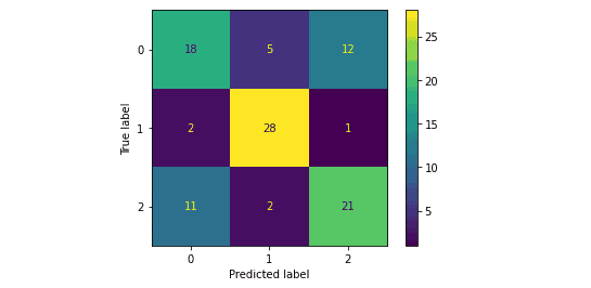
Notice that there were three output classes in our dataset, which is why there are three columns/rows in the confusion matrix.

Lose functions of the decision tree algorithm

The loss function is the error or mistakes the model has made while predicting. For example, if the true label is 0 or lost, but our model predicted it as 1 or winning, it made a mistake. As a result, our model loss increases. That means the less the loss function, the better model’s performance will be. Some of the loss functions are:

Log Loss: Log loss is also a logistic loss or cross-entropy loss.  Log Loss is the negative average of the log of corrected predicted probabilities for each instance.

Cohen Kappa: Cohen’s Kappa is a popular loss function robust for imbalanced datasets. Because, by default, it always searches for minor classes in the dataset.

Hinge Loss: Hinge loss is a specific cost function that incorporates a margin or distance from the classification boundary into the cost calculation.

Hamming Loss: Hamming loss is the fraction of wrong labels to the total number of labels. In multi-class classification, the hamming loss is calculated as the hamming distance between y_true and y_pred.

Let us now calculates the given loss functions of our trained model.

# importing the module
from sklearn.metrics import hamming_loss, hinge_loss, log_loss, cohen_kappa_score
# printing the loss functions
print(f'Log Loss: {log_loss(y_test, y_pred):.3f}')
print(f'Cohen Kappa: {cohen_kappa_score(y_test, y_pred):.3f}')
print(f'Hinge Loss: {hinge_loss(y_test, y_pred):.3f}')
print(f'Hamming Loss: {hamming_loss(y_test, y_pred):.3f}')

Output:

FAQ

Summary

A Decision Tree is one of the most powerful and popular algorithms for data classification and prediction. This article covered the Decision Tree theory and implementation using Python and AWS SageMaker Studio. In addition, we’ve covered the performance evaluation of the Decision Tree algorithm by using a confusion matrix, a matrix containing actual and predicted outputs. The confusion matrix helps us calculate the accuracy, precision, recall, and f1-score of binary and multi-class classification problems.