Introduction to Pandas DataFrames

Pandas is an open-source Python package based on NumPy widely used by data scientists for data analysis and manipulation. It provides ready-to-use high-performance data structures and data analysis tools. In Machine Learning, Pandas helps load, prepare, manipulate, model, and analyze the data before feeding this data to ML algorithms. This article will cover Pandas installation, basic DataFrames’ operations, data indexing, aggregation, and visualization.

Pandas help control and manipulate vast amounts of data. Whether the computing task is like finding the mean, median, and mode of data or processing large CSV files, Pandas is the package of choice.

Best Machine Learning Books for Beginners and Experts

As Machine Learning becomes more and more widespread, both beginners and experts need to stay up to date on the latest advancements. For beginners, check out the best Machine Learning books that can help to get a solid understanding of the basics. For experts, reading these books can help to keep pace with the ever-changing landscape. In either case, a few key reasons for checking out these books can be beneficial.

First, they provide a comprehensive overview of the subject matter, mainly about Machine Learning algorithms. Second, they offer insights from leading experts in the field. And third, they offer concrete advice on how to apply Machine Learning concepts in real-world scenarios. As Machine Learning continues to evolve, there’s no doubt that these books will continue to be essential resources for anyone with prior knowledge looking to stay ahead of the curve.

Installation

Pandas module is not available in the standard Python distribution, so we have to install it explicitly before using it. The most common way of installing the pandas module on your system is using the pip command. If you are using Jupyter notebook, run the following command in the cell of Jupyter Notebook to install it:

%pip install pandas

If you use any other IDE/text editor, open the terminal and use the following command to install Pandas:

pip install pandas

Once the installation is complete, we can check the version and details about the pandas module by typing the following commands:

pip show pandas

Output:

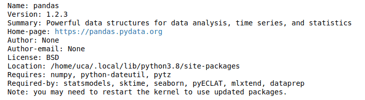
Now we can import the pandas module and start using it.

import pandas as pd

Importing different types of files

As we discussed, Pandas is a powerful and flexible Python package that allows you to work with labeled and time-series data. It also provides statistics methods, enables plotting, and more. One crucial feature of Pandas is its ability to write and read Excel, CSV, and many other types of files. Some of which we will discuss in this section.

Reading CSV files

The read_csv() function in Pandas helps you import and read the data in CSV format:

# importing csv dataset
dataset = pd.read_csv("myfile.csv")
#dataset showing
dataset

Output:

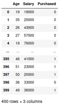
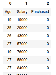
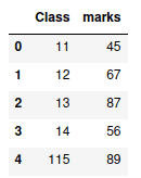
Notice that by default the read_csv() method considers the first row a header and sets auto-indexing for rows. We can change these default values to include the first row in our data and hide the auto-indexing for the rows.

# importing csv dataset, header = None
dataset = pd.read_csv("myfile.csv", header = None)
# hiding the indexing
dataset.style.hide_index()

Output:

Reading Excel files

You can use the read_excel() method to import and read Excel files:

# importing and reading xlsx file
dataset_excel = pd.read_excel("MyFile.xlsx")
dataset_excel

Output:

Excel organizes the data in one or more sheets. We can load data from the specific sheet by providing their names and the file name. For example, let’s access the data in Sheet2 of the Excel file:

# importing and reading xlsx file
dataset_excel = pd.read_excel("MyFile.xlsx", sheet_name="Sheet2")
dataset_excel

Output:

Reading JSON files

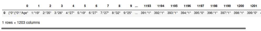
JSON stands for JavaScript Object Notation, a text format for storing and transmitting data between computer systems. The read_json() method in Pandas helps us import and read the data in JSON format:

# importing the JSON file
data_json = pd.read_csv("data_set.json", header=None)
# json dataset
data_json

Output:

Pandas support lots of other file types and data sources, for example, HD5, ORC, SQL, BigQuery, etc. Check out the official documentation for more information.

Pandas DataFrames

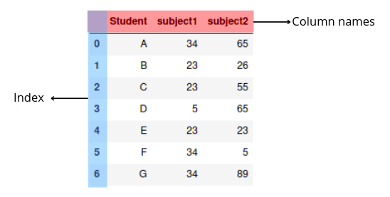
DataFrame in Pandas is a two-dimensional labeled data structure with columns of potentially different types. In general, we can say that Pandas DataFrame consists of three main components:

• columns
• index
• data

Here’s what the Pandas DataFrame looks like:

Creating DataFrame from Python dictionary

There are many ways to create Pandas DataFrames. One of the simplest ways is to use a Python dictionary. A dictionary is an unordered and mutable Python container that stores mappings of unique keys to values.

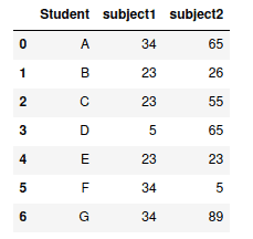
Let’s create a Python dictionary and convert it to Pandas DataFrame:

# creating dictionary
my_dict = {'Students': ["A", "B", "C", "D", "E"],
           "Subject1": [23, 45, 34, 22, 67],
           "Subject2": [67, 89, 66, 76, 54]}
# converting dict to pandas dataframe
my_dataframe = pd.DataFrame(my_dict)
# dataframe
my_dataframe

Output:

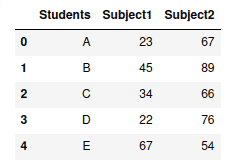
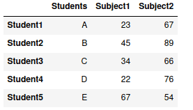
Notice that the indexing for the DataFrame has been done automatically. We can change the auto-indexing and introduce custom indexes:

# creating dictionary
my_dict = {'Students': ["A", "B", "C", "D", "E"],
           "Subject1": [23, 45, 34, 22, 67],
           "Subject2": [67, 89, 66, 76, 54] }
# converting dict to pandas dataframe
my_dataframe = pd.DataFrame(my_dict , index=["Student1", "Student2", "Student3", "Student4", "Student5"])
# dataframe
my_dataframe

Output:

Creating DataFrame from NumPy array

You can convert the NumPy array to Pandas DataFrame by passing it to the DataFrame class constructor. Let’s illustrate how to do it.

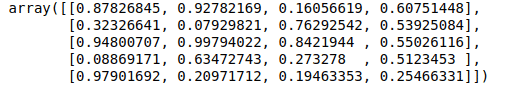
First, let’s create an array of random numbers using NumPy:

# importing numpy array
import numpy as np
# creating array of random numbers
narray = np.random.rand(5, 4)
# narray
narray

Output:

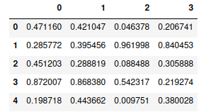
Now, we can convert the array to Pandas DataFrame:

# Pandas dataframe
my_dataframe = pd.DataFrame(narray)

# dataframe
my_dataframe

Output:

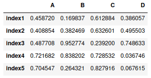
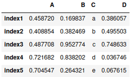
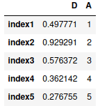
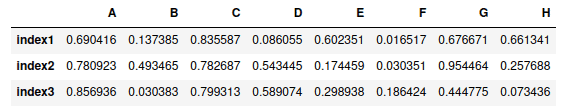
You can specify custom indexes and columns instead of using auto-indexing:

# Pandas dataframe
my_dataframe = pd.DataFrame(narray,
                            ["index1", "index2", "index3", "index4", "index5"], 
                            ["A", "B", "C", "D"])
# dataframe
my_dataframe

Output:

Accessing DataFrame columns

To access columns in DataFrame, you need to pass the column’s name inside the square brackets. Let’s access column C from the DataFrame:

# accessing column
column_c = my_dataframe['C']
# printing column
column_c

Output:

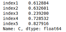
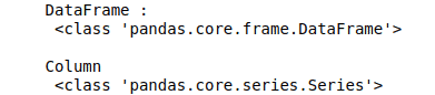
The output type is Pandas Series which is a one-dimensional labeled data structure. Every Pandas DataFrame is a collection of such Series.

# printing type of dataframe
print("DataFrame :\n", type(my_dataframe))
# pritning type of column
print("\nColumn\n", type(column_c))

Output:

Changing column’s values in DataFrame

You can change values in the DataFrame column by replacing values in the column’s Series. For example, let’s change values in column C:

# accessing column
my_dataframe['C'] = ['a', 'b', 'c', 'd', 'e']
# printing column
my_dataframe

Output:

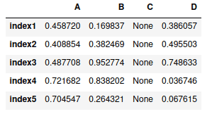
You can assign a single value to the entire column. For example, let’s change all values of column C to None.

# changing values
my_dataframe["C"] = None
# printing column
my_dataframe

Output:

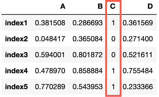
Finally, you can define a function to update values based on your conditions:

# creating array of random numbers
narray = np.random.rand(5, 4)
# defining Pandas DataFrame
my_dataframe = pd.DataFrame(narray,
                            ["index1", "index2", "index3", "index4", "index5"], 
                            ["A", "B", "C", "D"])
# function for conditional updates
def update_column(val):
    if val < 0.5:
        return 0
    else:
        return 1
# update DataFrame column based on condition
my_dataframe['C'] = my_dataframe.apply(lambda x: update_column(x['C']), axis=1)
my_dataframe

Output:

For more information about conditional updates in Pandas DataFrame check out the 5 ways to apply an IF condition in the Pandas DataFrame article.

Deleting DataFrame column

To delete the column from the Pandas DataFrame, you need to use the drop() DataFrame’s built-in function. For example, let’s drop column C from the DataFrame:

# droping column
data_set = my_dataframe.drop("C", axis=1)
# printing
print("original dataframe\n", my_dataframe)
print("\ncolum deleted\n", data_set)

Output:

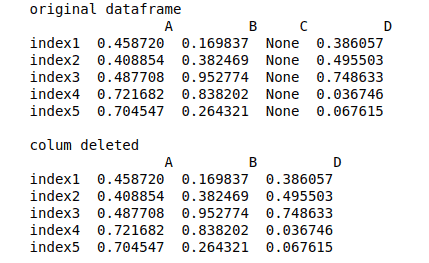
Note that we have assigned 1 to the axis, which means dropping the column named “C” from the columns. If we assign zero to the axis, then it will drop the row. Another thing to notice is that the column is not dropped from the original DataFrame, so if we want to remove the column from the original DataFrame, then we have to assign True for inplace parameter:

# droping column completly
my_dataframe.drop("C", axis=1, inplace = True)
# printing
print("original dataframe\n", my_dataframe)

Output:

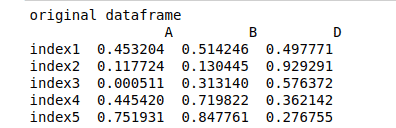
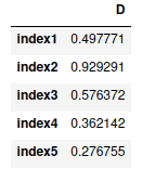
You can also delete multiple columns by passing a list of columns. For example, let’s delete columns A and B from the DataFrame:

# droping column completly
my_dataframe.drop(["A","B"] , axis=1, inplace= True)
# printing
my_dataframe

Output:

Adding column to the DataFrame

To add a new column to DataFrame, you need to create a new list of values and then assign it to the DataFrame by specifying the column name. For example, let’s add a new column “A” to the DataFrame:

# creating list 
mylist = [1,2,3,4,5]
# adding column to dataframe
my_dataframe['A'] = mylist
# printing
my_dataframe

Output:

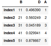
Another method of adding a new column to the DataFrame is to use the insert() method, which allows adding a column at any position within the DataFrame. Let’s add column “C” to DataFrame as the first column:

# creating list 
mylist1 = [11,21,31,41,51]
# adding column to dataframe
my_dataframe.insert(0, "B", mylist1, True)
# printing
my_dataframe

Output:

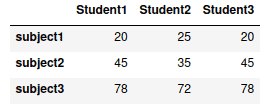
Pandas DataFrame with nested dictionaries

A nested dictionary is a Python dictionary inside a dictionary. You can create a Pandas DataFrame from a nested dictionary. The keys of the outer dictionary will be considered as column names, and the keys of the inner dictionaries will be considered as the index of the rows:

# creating dictionary
dict = {'Student1': {"subject1": 20, "subject2": 45, "subject3": 78},
        'Student2': {"subject1": 25, "subject2": 35, "subject3": 72},
        'Student3': {"subject1": 20, "subject2": 45, "subject3": 78},
       }
# converting nested dict to DataFrame
data_frame=pd.DataFrame(dict)
# printing
data_frame

Output:

Now, let’s see what will happen if we convert a nested dictionary having different “keys” names to DataFrame.

# creating dictionary
dict = {'Student1': {"Math": 20, "English": 45, "Urdu": 78},
        'Student2': {"Physics": 25, "Computer": 35, "Finance": 72},
        'Student3': {"Java": 20, "Python": 45, "Statistic": 78},
       }
# converting nested dict to DataFrame
data_frame=pd.DataFrame(dict)
# printing
data_frame

Output:

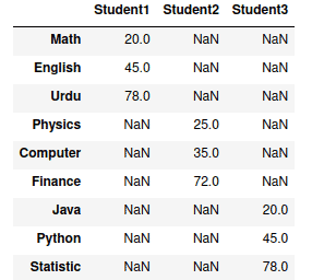
Note that Pandas created a new row for each of the unique keys and assigned “NaN” to the missing values.

Working with NULL values in DataFrame

Missing values in Pandas Dataframes are represented using NaN. Missing data can occur when no information is provided for one or more items or a whole unit. There are many built-in methods in pandas to work and handle null values.

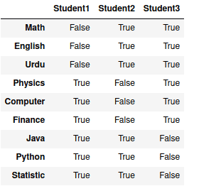
For example, the isnull() method returns True wherever Null value appears in the DataFrame. Let’s take the previous Dataframe and apply isnull() method:

# appling isnull() method
data_frame.isnull()

Output:

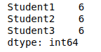
You can find the total number of null values in each column by using isnull().sum() methods combination:

# finding total null values
data_frame.isnull().sum()

Output:

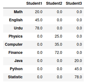
We can also fill the null value with other values by using the fillna() method.

# filling null values with zero
data_frame.fillna(0)

Output:

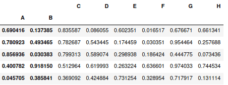
Indexing and selecting data

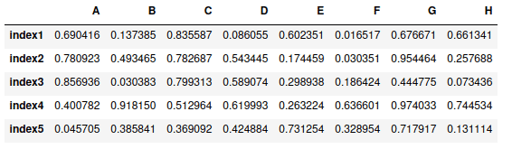
Pandas have many build-in methods for indexing and selecting specific data from DataFrame. Let’s create a random DataFrame and then apply different methods for selecting the data:

# creating array of random numbers
narray = np.random.rand(5, 8)
# narray
narray
# Pandas dataframe
my_dataframe = pd.DataFrame(narray ,
                            ["index1", "index2", "index3", "index4", "index5"], 
                            ["A", "B", "C", "D", "E", "F", "G", "H"])

# dataframe
my_dataframe

Output:

loc[] – selection by index name

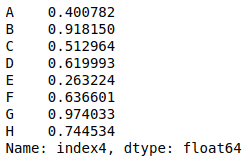
The DataFrame’s loc[] indexer allows you to select rows by labels or by boolean condition. For example, let’s select the row having index “index4”:

# selecting specific row
my_dataframe.loc["index4"]

Output:

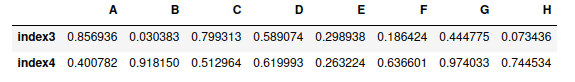
You can use the same method to select multiple rows by using two square brackets instead of single brackets. For example, let’s select rows having “index3” and “index4” from the DataFrame:

# selecting specific rows
my_dataframe.loc[["index3","index4"]]

Output:

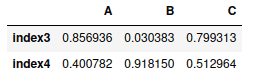
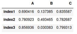
The loc[] is not only used to select rows but it can be used to select rows from custom columns:

# selecting specific data
my_dataframe.loc[['index3', 'index4'], ['A', 'B', 'C']]

Output:

iloc[ ] – selection based on index position

The iloc[] indexer for Pandas DataFrame is used for integer location-based indexing/selection by position. Instead of taking the names of rows and columns, this method takes the index values of column and row.

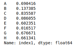
For example, let’s select the first row using this method.

# selecting row using iloc
my_dataframe.iloc[0]

Output:

Panadas also help us to slice the DataFrame and select multiple rows. For example, let’s select the first three rows of the DataFrame:

# selecting row using iloc
my_dataframe.iloc[0:3]

Output:

The important thing about iloc[] is that you can select the column’s index positions too. For example, let’s select the data from the first three rows and columns:

# selecting rows using iloc
my_dataframe.iloc[0:3, 0:3]

Output:

Multi-indexing in DataFrame

Multi-indexing is when we assign more than one labeled indexes values to the DataFrame. For example, let’s say we have the DataFrame and we want to use columns A and B as the indexes for the DataFrames’ rows:

# creating multi-indexing
my_dataframe.set_index(["A","B"], inplace=True)
my_dataframe

Output:

Now we can select the row using different index values (values of the A and B column or Python indexing).

my_dataframe.loc[(0.9717886841828848, 0.8169436261887079)]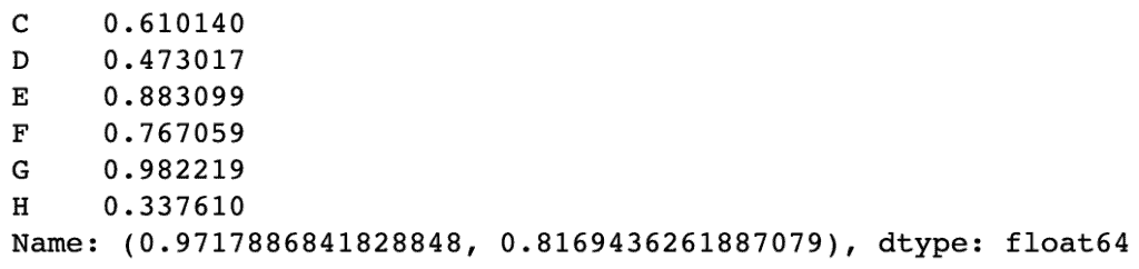

Note: In our example, DataFrame does not print complete index values in its table output. To see complete index values, use the DataFrame.index attribute:

my_dataframe.index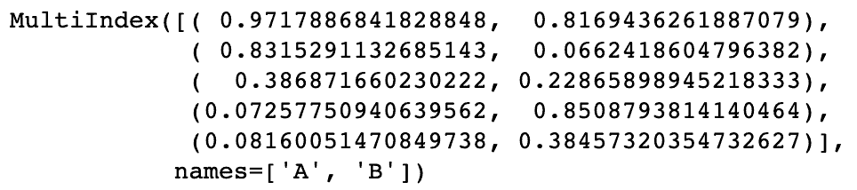

Merging and joining DataFrames

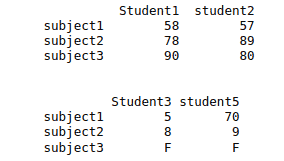
Pandas’ merging and joining functions allow combining different datasets to analyze data more efficiently. In the following examples, we will use various Pandas’ built-in methods to merge DataFrames, but let’s create two DataFrames first:

my_dataframe1 = pd.DataFrame({"Student1": {"subject1": 58, "subject2":78, "subject3":90}, 
                             "student2":{"subject1": 57, "subject2": 89, "subject3":80}})

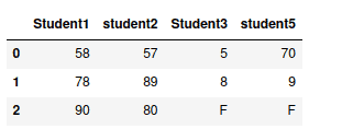
my_dataframe2 = pd.DataFrame({"Student3": {"subject1": 5, "subject2":8, "subject3":"F"}, 
                             "student5":{"subject1": 70, "subject2": 9, "subject3":"F"}})
# printing dataframes
print(my_dataframe1)
print("\n")
print(my_dataframe2)

Output:

DataFrames concatenation

The Pandas’ concat() method concatenates two DataFrame together:

# concatenating the dataframes
concat_dataframe = pd.concat([my_dataframe1, my_dataframe2])
# printing 
concat_dataframe

Output:

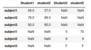
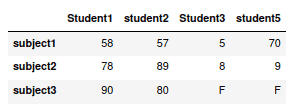
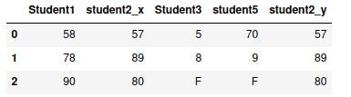
Notice that the DataFrames have been concatenated in vertical order. To concatenate them in horizontal order, we have to specify the axis argument:

# concatenating the dataframes
concat_dataframe = pd.concat([my_dataframe1, my_dataframe2], axis=1)
# printing 
concat_dataframe

Output:

Joining DataFrames

The Pandas merge() function allows joining (similar to SQL join expression) DataFrames with by common elements from the specified columns. This is achieved by the parameter “on” which allows us to select the common column between two DataFrames.

For example, we will merge the concat_dataframe and my_dataframe1 DataFrames based on Student1 column values:

# merging two dataframes
merged = pd.merge(concat_dataframe, my_dataframe1, on="Student1")
# printing
merged

Output:

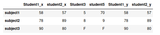
We can also merge the DataFrames based on multiple columns. For example, this time, we will join the DataFrame based on student1 and student2:

# merging two dataframes
merged = pd.merge(concat_dataframe, my_dataframe1, on=["Student1", "student2"])
# printing
merged

Output:

Moreover, we can also merge DataFrames based on indexing as well.

# merging two dataframes
merged = pd.merge(concat_dataframe, my_dataframe1, right_index= True, left_index = True)
# printing
merged

Output:

Aggregation and grouping in pandas DataFrame

Aggregation in Pandas provides various functions that perform a mathematical or logical operation on our dataset and returns a summary of that function. The most common aggregation functions are a simple average or summation of values. Generally, an aggregation function takes multiple individual values and returns a summary. You can use aggregation to get an overview of columns in our dataset, like getting sum, minimum, maximum, etc., from a particular column of our dataset.

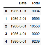
Let’s apply various aggregation and grouping methods to the following dataset:

import io
import requests
s=requests.get("https://hands-on.cloud/wp-content/uploads/2022/02/catfish_sales_1986_2001.csv").content
data=pd.read_csv(io.StringIO(s.decode('utf-8')))
data.head(5)

Output:

Count method

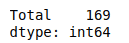
The Series’ count() function returns the number of entries for every column. Let’s get the total number of entries of the Total column from the dataset.

# count of the total column
data[["Total"]].count()

Output:

We can also find the total number of entries without using the square brackets.

# count of the total column
data.Total.count()

Output:

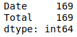
If we do not specify the column’s name, then the count method will return the total number of entries in each of the columns.

# count of the columns
data.count()

Output:

Sum method

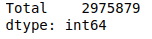
The Series’ sum() function helps to find the sum of elements in a column. For example, let us find the total sum of the entries in the Total column.

# sum method on Total column
data[["Total"]].sum()

Output:

Similarly, we can find the sum of the entries without using the square brackets.

# sum method on Total column
data.Total.sum()

Output:

One of the important usage of the sum() method in machine learning and data science is used to find the total number of NULL values from the dataset.

# finding the total null values
data.isnull().sum()

Output:

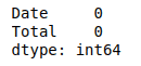
Fortunately, this dataset does not have any NULL values.

Min and Max methods

The min() and max() methods are used to find the minimum and maximum values from the DataFrame.

For example, we will find the minimum and maximum values from the Total column.

# minimum value
print("minimum value is :", data.Total.min())
# maximum value
print("maximum value is :", data.Total.max())

Output:

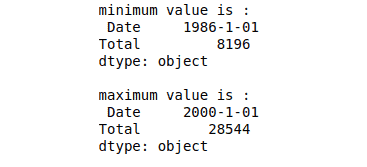
If we will not specify the column, then the min() and max() methods will return the minimum and maximum values from each of the columns.

# minimum value
print("minimum value is :\n", data.min())
# maximum value
print("\nmaximum value is :\n", data.max())

Output:

Mean and Median

The functions of the mean() and median() are to find the mean and median. The mean is the average, and the median is the middle value in a list ordered from.

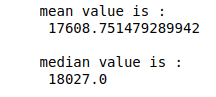
Let us find the mean and median of the Total column from the DataFrame.

# mean value
print("mean value is :\n", data.Total.mean())
# median value
print("\nmedian value is :\n", data.Total.median())

Output:

If we do not specify the column name, then the mean and median functions will return the mean and median of each column in the DataFrame.

Visualization of DataFrame

One of the essential things in Machine Learning and Data Science is to show the results in the visualized form. Data visualization helps us understand how data is used in a particular dataset. For example, in the above section, we had found the mean and median but didn’t know exactly where they lie in the dataset.

Visualize DataFrame mean and median

Let’s visualize the mean and median that we have just calculated.

# importing plolty graph
import plotly.graph_objects as go
fig = go.Figure()
# creating mean list
mean=[]
for i in range(len(data['Date'])):
    mean.append(data.Total.mean())
    
# creating median list
median = []
for i in range(len(data['Date'])):
    median.append(data.Total.median())
    
# ploting mean
fig.add_trace(go.Scatter(x=data['Date'], y=mean,
                    mode='lines',
                    name='Mean'))
# ploting median
fig.add_trace(go.Scatter(x=data['Date'], y=median,
                    mode='lines',
                    name='Media'))
# ploting data
fig.add_trace(go.Scatter(x=data['Date'], y=data["Total"],
                    mode='lines',
                    name='Data'))

Output:

Visualize DataFrame using histogram

A Histogram is a variation of a bar chart in which data values are grouped and put into different classes. This grouping enables us to see how frequently data in each class occur in the dataset.

Let’s now visualize the DataFrame using the histogram:

# importing the module
import plotly.express as px
# ploting the bar graph
fig = px.bar(data, x=data['Date'], y=data['Total'])
fig.show()

Output:

Visualizing DataFrame using line chart

Line graphs are used to track changes over short and long periods. When more minor changes exist, line graphs are better than bar graphs. You can also use line graphs to compare changes for more than one group over the same period.

Let’s visualize the DataFrame using the line chart.

# importing plolty graph
import plotly.graph_objects as go
fig = go.Figure()
# ploting data
fig.add_trace(go.Scatter(x=data['Date'], y=data["Total"],
                    mode='lines+markers',
                    name='Data'))
fig.show()

Output:

Visualizig DataFrame using Scattered plot

A scatter plot is a type of data visualization that shows the relationship between different variables. This data is shown by placing various points between an x- and y-axis. Essentially, each of these data points looks “scattered” around the graph. A scattered graph helps us visualize the relationship (especially clusters) and outliers present in our dataset.

Let’s now visualize the DataFrame using a scattered graph.

# ploting
fig = go.Figure()
# ploting data
fig.add_trace(go.Scatter(x=data['Date'], y=data["Total"],
                    mode='markers',
                    name='Data'))
fig.show()

Output:

Visualizing DataFrame using box-plot

A box plot is a simple way of representing statistical data on a plot in which a rectangle is drawn to represent the second and third quartiles, usually with a vertical line inside to indicate the median value. The lower and upper quartiles are shown as horizontal lines on either side of the rectangle. Box plots are helpful as they provide a visual summary of the data enabling researchers to quickly identify mean values, the dispersion of the data set, and signs of skewness.

Let’s use the box-plot to plot our DataFrame.

# importing module
import plotly.express as px
# ploting bo plot
df = px.data.tips()
fig = px.box(df, y=data["Total"])
fig.show()

Output:

Summary

Pandas is an open-source Python package based on NumPy widely used by data scientists for data analysis and manipulation. Pandas help load, prepare, manipulate, model, and analyze the data before feeding this data to ML algorithms. This article covered Pandas installation, basic DataFrames’ operations, data indexing, aggregation, and visualization.