SageMaker Canvas: Simple Time-series Forecasting

Time-series forecasting is a challenging, compute, and time-consuming task, which is hard to implement to achieve accurate results. At re:Invent2021 Amazon announced the Amazon SageMaker Canvas service that gives you the ability to use Machine Learning to generate predictions without code. This article will cover how to use Amazon SageMaker Canvas to create a forecasting model and make predictions for time-series datasets.

In this article, we’ll load Amazon stock historical data, prepare it for Amazon SageMaker Canvas, run Canvas workflow, import predictions data back, and compare it with real stock future data and SARIMA algorithm predictions.

We highly recommend you check out the Time Series Forecasting Principles with Amazon Forecast guide as soon as Amazon SageMaker Canvas uses Amazon Forecast to make predictions out of time-series datasets.

Best Machine Learning Books for Beginners and Experts

As Machine Learning becomes more and more widespread, both beginners and experts need to stay up to date on the latest advancements. For beginners, check out the best Machine Learning books that can help to get a solid understanding of the basics. For experts, reading these books can help to keep pace with the ever-changing landscape. In either case, a few key reasons for checking out these books can be beneficial.

First, they provide a comprehensive overview of the subject matter, mainly about Machine Learning algorithms. Second, they offer insights from leading experts in the field. And third, they offer concrete advice on how to apply Machine Learning concepts in real-world scenarios. As Machine Learning continues to evolve, there’s no doubt that these books will continue to be essential resources for anyone with prior knowledge looking to stay ahead of the curve.

Requirements

For demo purposes, we’ll use the following Python modules:

• pandas – a fast, powerful, flexible, and easy to use open-source data analysis and manipulation tool
• plotly – a data analytics and visualization library
• pandas_datareader – a remote data access module for pandas that allows reading data from various sources
• statsmodels – this module provides classes and functions for the estimation of many different statistical models (we’ll use its SARIMA algorithm implementation)

You can install the required dependencies by executing the following code in your Jupyter notebook:

%pip install pandas
%pip install pandas_datareader
%pip install plotly
%pip install statsmodels

Loading dataset

As a time-series dataset, we’ll take Amazon stocks data from 2008-01-01 to 2022-02-09 and try to make predictions for the next couple of days.

To load historical stock data, we’ll use the pandas_datareader module:

from pandas_datareader import data
start_date = '2008-01-07'
end_date = '2022-02-09'
stock_data = data.get_data_yahoo('AMZN', start_date, end_date)
stock_data.head(10)

As a result, we’ll get a pandas DataFrame named stock_data:

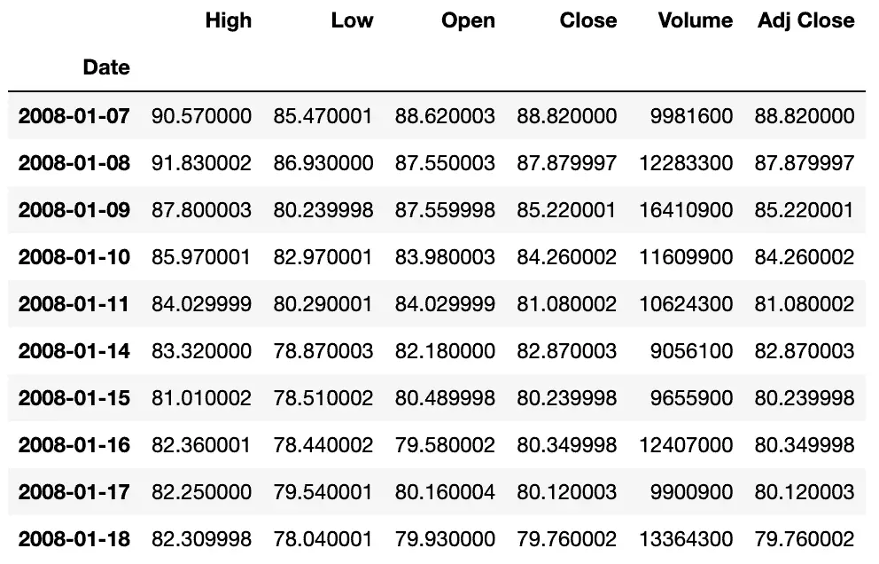
Let’s visualize the dataset using Plotly:

import pandas as pd
pd.options.plotting.backend = "plotly"
columns = ['High', 'Low', 'Open', 'Close', 'Adj Close']
fig = stock_data[columns].plot()
fig.update_layout(title_text=f"Amazon stocks historical data: {start_date} - {end_date}")
fig.show()

Preparing dataset for Amazon SageMaker Canvas

Next, we need to prepare our time-series dataset for Amazon SageMaker Canvas.

The Amazon SageMaker Canvas has several requirements for the dataset:

• Column to predict – The column that contains examples of data for forecasting
• Item ID column – The column that contains unique identifiers for each item in your dataset. In our example, a number uniquely identifies the stock
• Timestamp column – The column containing the timestamps in your dataset (Format: yyyy-MM-dd HH:mm:ss)

For additional information about the model configuration, check out the Make a time series forecast documentation.

We’ll use the period’s close price (the Close column) to predict the stock price. Let’s drop unnecessary columns from the dataset and add the Amazon stock index (we’ll use 0, for example).

# create a copy of the dataframe
df = stock_data.copy()
# add column with unique identifier for the stock
df['ID'] = 0
# reindex dataframe to the datetime
# format required by AWS SageMaker Canvas (yyyy-MM-dd HH:mm:ss)
df.index = df.index.strftime('%Y-%m-%d %H:%M:%S')
# setting up dataframe index as a column
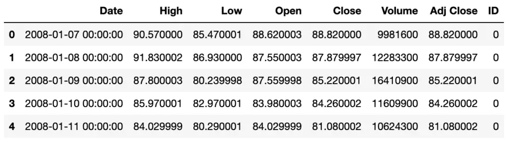
df = df.reset_index()
df.head()

Now, our dataset looks like this:

Let’s save our dataset for Amazon SageMaker Canvas:

df.to_csv(f'amazon_stock_daily_{start_date}_{end_date}.csv', index=False)

Amazon SageMaker Canvas workflow

In this section of the article, we’ll import the prepared dataset to Amazon SageMaker Canvas, run its workflow, generate predictions, and export them back to the Jupyter Notebook for comparison with the SARIMA algorithm predictions and actual stock values.

Creating model

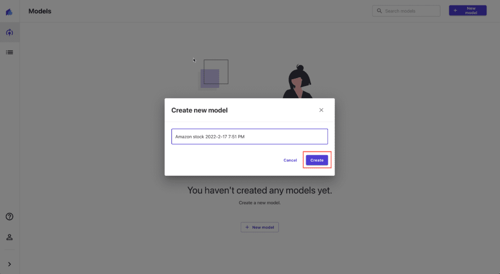
First, we need to open Amazon SageMaker Canvas and press the New Model button:

Provide the new model name (do not use brackets or quotes, as that will cause strange hard to investigate issues at the build step later):

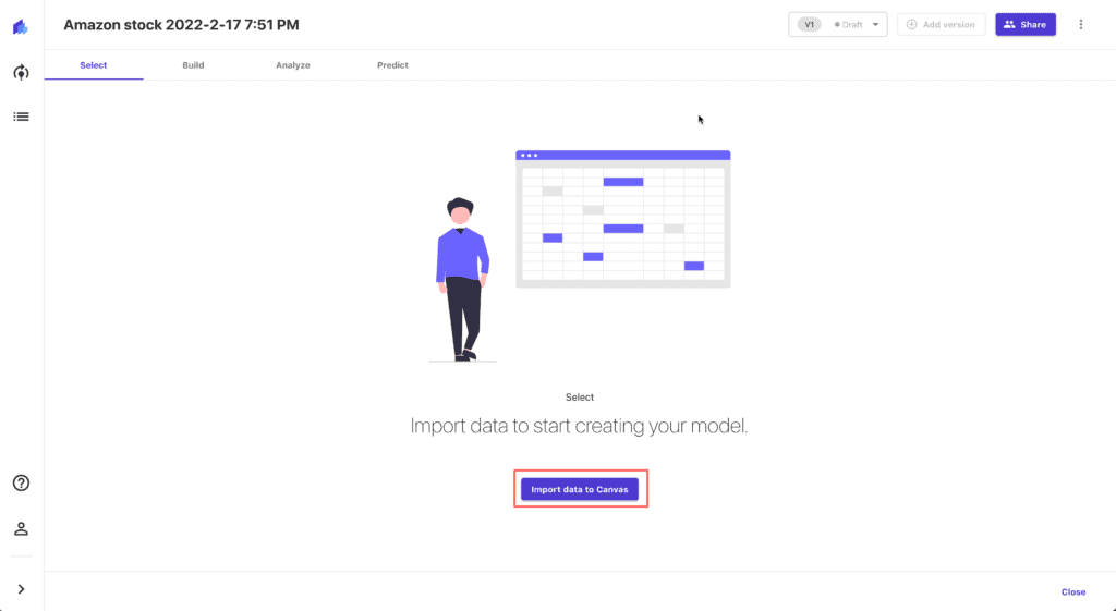
Importing dataset

Press the Import data to Canvas to start importing process:

Upload the CSV file from your laptop (you can use the S3 bucket as your data source too):

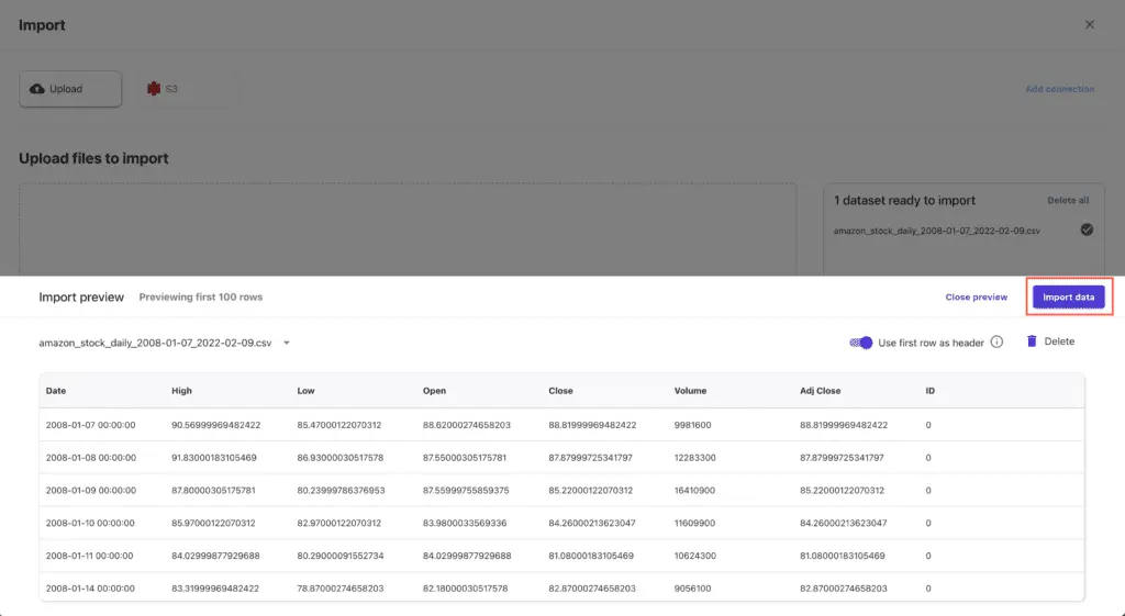
Preview the imported data:

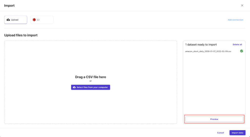
If everything’s OK, hit the Import data button:

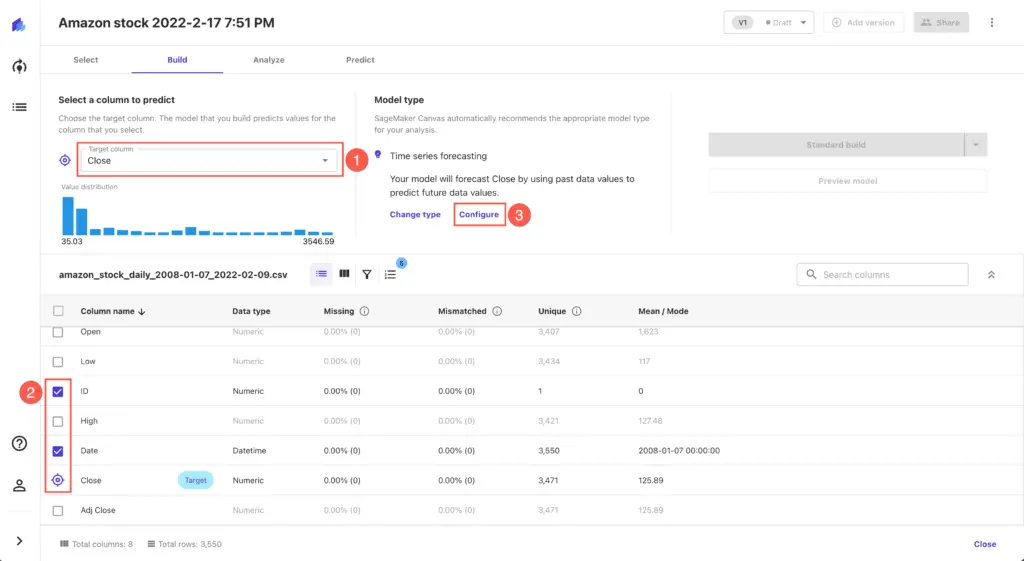
Building the model

To build the model, we need to configure it first. Set Target column value to Close and make sure that only ID and Date columns are selected in the columns list. Press Configure link to set up model configuration.

Set up the following parameters for the time series forecasting configuration:

• Item ID column: ID
• Timestamp column: Date
• Duration: the number of days you’re willing to get predictions for (we’ll use 10)
• Use holiday schedule: United States

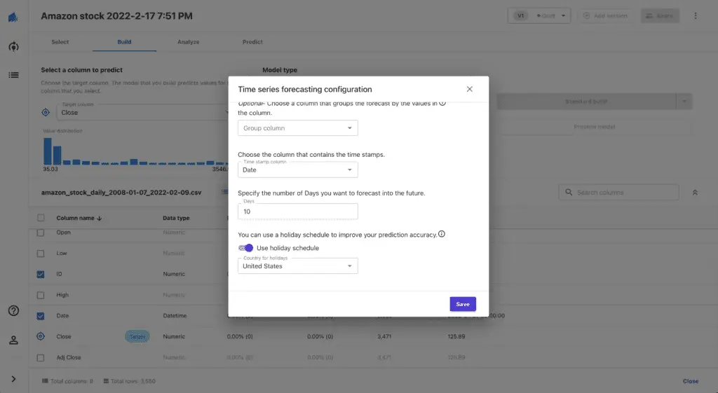
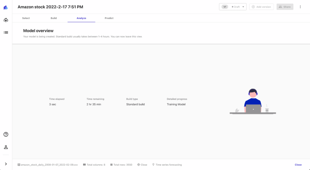
Hit the Save button and start the model build process by pressing the Standard build button.

The process will take a couple of hours. It’s time for a coffee break.

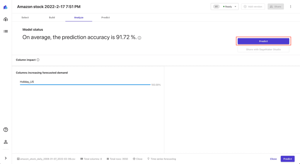
Generating predictions

As soon as the model build process is complete, press the Predict button:

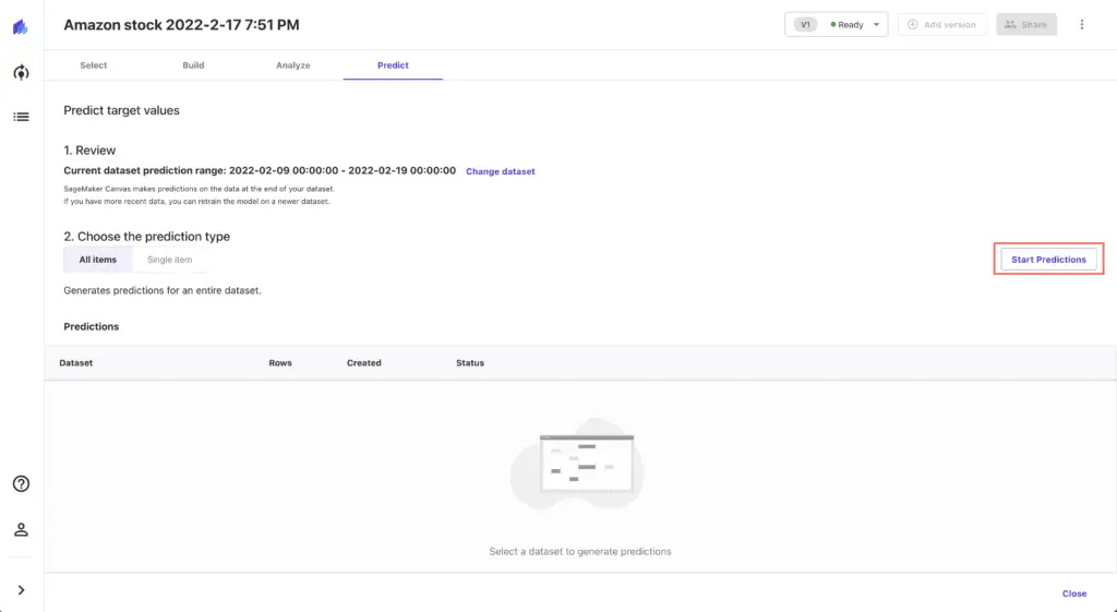
Press the Start predictions button to generate forecasted values (the process will take several minutes):

Download the generated predictions CSV file and upload it to your Jupyter Studio:

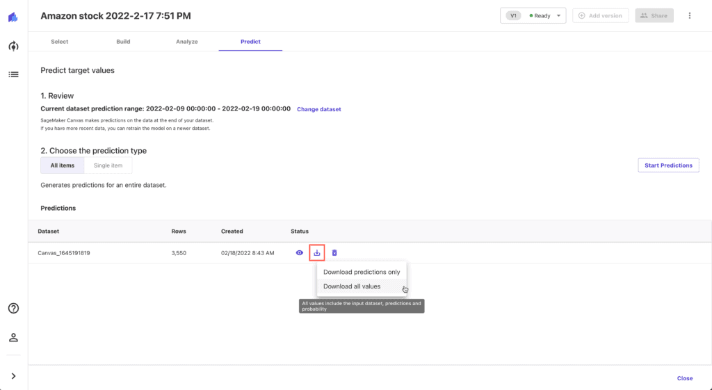
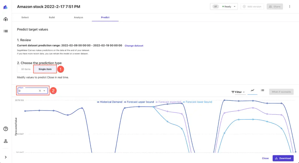
While Amazon SageMaker Canvas generates the file, you can review forecasts by clicking on the Single item prediction type:

Importing data to Jupyrer Notebook

To import the Amazon SageMaker Canvas predictions to Jupyter Notebook, use the following code:

# loading data from CSV file
canvas_predictions = pd.read_csv('Canvas_1645191819_2022-02-18T13-58-30Z_part0.csv')
# droping ID column (we con't need it)
canvas_predictions.drop(['ID'], axis=True, inplace=True)
# setting up Date column as a new index
canvas_predictions= canvas_predictions.set_index('Date')
# removing weekend datapoints with negative values from the dataset
canvas_predictions = canvas_predictions[canvas_predictions.p10 > 0]
canvas_predictions = canvas_predictions[canvas_predictions.p50 > 0]
canvas_predictions = canvas_predictions[canvas_predictions.p90 > 0]
canvas_predictions.head()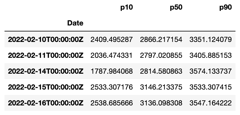

Let’s quickly visualize a part of this dataset:

pd.options.plotting.backend = "plotly"
canvas_predictions['2022-02-10':'2022-02-16'].plot()

Generating predictions using SARIMA algorithm

Let’s generate our predictions using the SARIMA algorithm.

First, let’s check out which model parameters works better. To list all possible combinations, run the following code:

import itertools
p = d = q = range(0, 2)
pdq = list(itertools.product(p, d, q))
seasonal_pdq = [(x[0], x[1], x[2], 5) for x in list(itertools.product(p, d, q))]
print('Examples of parameter for SARIMA...')
print('SARIMAX: {} x {}'.format(pdq[1], seasonal_pdq[1]))
print('SARIMAX: {} x {}'.format(pdq[1], seasonal_pdq[2]))
print('SARIMAX: {} x {}'.format(pdq[2], seasonal_pdq[3]))
print('SARIMAX: {} x {}'.format(pdq[2], seasonal_pdq[4]))

Now, we can run the SARIMA algorithm with all varieties of parameters and choose the best one (minimal Akaike Information Criterion value):

import statsmodels.api as sm
close = stock_data['Close'].copy()
close.index = pd.DatetimeIndex(close.index).to_period('d')
params = {'param': None, 'param_seasonal': None, 'lowest': None}
for param in pdq:
    for param_seasonal in seasonal_pdq:
        try:
            mod = sm.tsa.statespace.SARIMAX(close, order=param, seasonal_order=param_seasonal, enforce_stationarity=False, enforce_invertibility=False)
            results = mod.fit()
            if params['lowest'] == None:
                params = {'param': param, 'param_seasonal': param_seasonal, 'lowest': results.aic}
            else:
                if results.aic < params['lowest']:
                    params = {'param': param, 'param_seasonal': param_seasonal, 'lowest': results.aic}
        except:
            continue
print('====> SARIMA{}x{}5 - AIC:{}'.format(params['param'],params['param_seasonal'], params['lowest']))

After that, we can execute the SARIMA algorithm with the best working parameters and print the summary:

mod = sm.tsa.statespace.SARIMAX(close,
                                order=params['param'],
                                seasonal_order=params['param_seasonal'],
                                enforce_stationarity=False,
                                enforce_invertibility=False)
results = mod.fit()
print(results.summary().tables[1])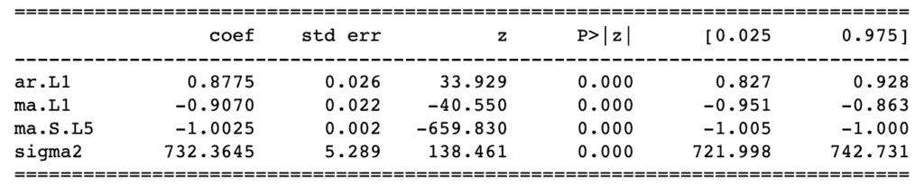

Now, we can generate SARIMA predictions DataFrame. Please, pay attention that we’ve adjusted start_date, as soon as the SARIMA algorithm requires at least one data point from the original dataset:

start_date = '2022-02-09'
end_date = '2022-02-16'
pred = results.get_prediction(start=pd.to_datetime(start_date), end_date=pd.to_datetime(end_date), dynamic=False)
pred_ci = pred.conf_int()
pred_uc = results.get_forecast(steps=7)
pred_ci = pred_uc.conf_int()
sarimax_predictions = pd.DataFrame(
    {
        'Sarimax': pred_uc.predicted_mean,
        'Date': pd.date_range(start='02/10/2022', periods=7, freq='D')
    }
)
sarimax_predictions.set_index("Date", inplace=True)
sarimax_predictions.head()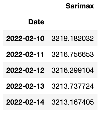

Comparing results

Let’s load additional stock values and compare Amazon SageMaker Canvas and SARIMA algorithm predictions with the actual stock values:

start_date = '2022-02-10'
end_date = '2022-02-16'
stock_data_extended = data.get_data_yahoo('AMZN', start_date, end_date)
stock_data_extended = stock_data_extended[start_date:end_date]
stock_data_extended.head()

Let’s select only required data from the Amazon SageMaker Canvas DataFrame for the date range we’re interested in:

start_date = '2022-02-10'
end_date = '2022-02-17'
canvas_predictions = canvas_predictions[start_date:end_date]

Now, we can put all data points to the same plot to see the results:

import plotly.graph_objects as go
fig = go.Figure()
fig.add_trace(go.Scatter(x=stock_data_extended.index.astype(str), y=stock_data_extended['Close'],
                    mode='lines',
                    name='Real values'))
fig.add_trace(go.Scatter(x=canvas_predictions.index.astype(str), y=canvas_predictions['p10'],
                    mode='lines',
                    name='Predicted (p10)'))
fig.add_trace(go.Scatter(x=canvas_predictions.index.astype(str), y=canvas_predictions['p50'],
                    mode='lines',
                    name='Predicted (p50)'))
fig.add_trace(go.Scatter(x=canvas_predictions.index.astype(str), y=canvas_