Implementation of AdaBoost algorithm using Python

Boosting algorithms are an ensemble learning technique that allows the merging of different simple models to generate the ultimate model output. Instead of using just one model on a dataset, boosting algorithm can combine models and apply them to the dataset, taking the average of the predictions made by all the models. In this process, all models are trained sequentially so that each model tries to compensate weaknesses of its predecessor. In this article, we will cover the AdaBoost algorithm implementation for solving classification and regression problems. We will use Amazon SageMaker and Jupyter notebooks for implementation and visualization purposes.

AdaBoost (Adaptive Boosting) algorithm is a statistical classification meta-algorithm algorithm initially created to increase the efficiency of binary classifiers. At the same time, you can use AdaBoost to boost the performance of any Machine Learning algorithm.

Before moving ahead, make sure that you have a solid understanding of Decision Trees and Random Forest because we will use these algorithms to get better predictions on the training dataset.

Best Machine Learning Books for Beginners and Experts

As Machine Learning becomes more and more widespread, both beginners and experts need to stay up to date on the latest advancements. For beginners, check out the best Machine Learning books that can help to get a solid understanding of the basics. For experts, reading these books can help to keep pace with the ever-changing landscape. In either case, a few key reasons for checking out these books can be beneficial.

First, they provide a comprehensive overview of the subject matter, mainly about Machine Learning algorithms. Second, they offer insights from leading experts in the field. And third, they offer concrete advice on how to apply Machine Learning concepts in real-world scenarios. As Machine Learning continues to evolve, there’s no doubt that these books will continue to be essential resources for anyone with prior knowledge looking to stay ahead of the curve.

Explanation of AdaBoost algorithm

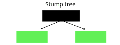
AdaBoost (also called Adaptive Boosting) is an ensemble method technique in Machine Learning that combines several base models in order to produce one optimal predictive model. The AdaBoost can use any classifier making weak predictions and combine them to build a strong predictive model. The most popular classifier used by AdaBoost algorithm is Decision Trees with one level (the Decision Trees does only 1 split). These trees are called Decision Stumps which are similar to Random Forest trees, but not “fully grown.”

The three most important ideas behind the AdaBoost algorithm using Decision Trees are:

• AdaBoost combines a lot of week learners to make better predictions which are known as stumps
• Some stumps have more contribution to the predictions than others
• Each stump tree is considering the previous stump’s mistakes into account

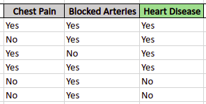
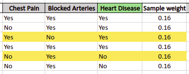
To understand how the AdaBoost algorithm works, we will take a sample dataset that contains data about whether a patient has heart disease or not depending on some input variables. And we will also restrict the AdaBoost algorithm to be trained on only one stump tree.

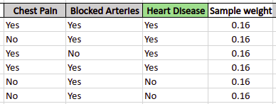
The first step is to assign weights to each of the samples (patients). At this step, the algorithm assigns the same weight to each of the samples because for the first iteration all samples all are equally important. The weight is assigned to each of the samples using the following formula:

sample weight = 1 / total samples

In our case, there is a total of 6 samples, so the weight of each sample will be ~0.16.

After assigning weights, the AdaBoost will use a Decision Tree is to create stumps trees based on the given dataset. In our case, 2 stumps trees will be created as we have two input variables.

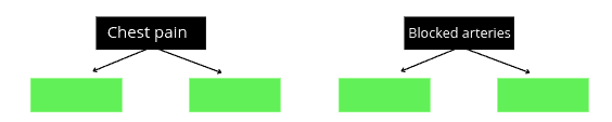
Based on the entropy value, the AdaBoost algorithm will select the stump tree that has lower entropy value. Let’s say the Chest pain stump tree has less entropy value so our model will select it as a base learning model.

In the next step, the AdaBoost will compare the predictions of the chest pain stump tree with the actual values from the training dataset to calculate the classification error.

Let’s say, the stump tree misclassified 2 out of 6 input data (highlighted below):

As soon as there were two misclassifications, the total error is:

Total error = misclassified/total samples

Total error = 2/6 = 0.333

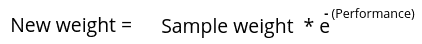
The third step is finding the performance of the stump tree. The Adaboost algorithm will use the following formula to calculate the performance of the stump:

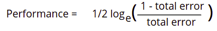
We get 0.3466 as the performance rate of our model.

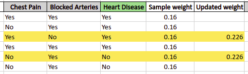
The next step is to update the sample weights on the dataset based on the performance of the stump. The algorithm will increase weights for samples that being incorrectly classified and decrease weights of samples which were classified correctly, and the next stump tree will know about the misclassified samples.

The formula to update the weights of misclassified data is:

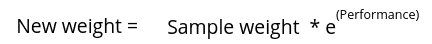
Using the above formula, the new weight assigned to misclassified samples will be:

The next step is to update the correctly classified samples using slightly different formula:

So, the newly assigned weights to the correctly classified samples will be:

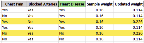
The misclassified sample’s weight had increased and the correctly classified sample’s weight has been decreased as compared to their initial weight. So, for the samples, that would have a weight greater than their previous weight, the next stump tree will “understand” that these were misclassified by the previous stump and will try to reduce their weight by classifying them correctly.

Before building the next stump tree, the algorithm normalizes the updated weights so that their sum becomes equal to 1. The following formula is used to normalize the updated weight:

Normalized weight = Updated weight / sum of total weights

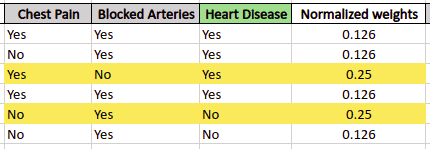
The next stump tree will use these normalized weights for the training and making predictions.

Because we restricted the model to have only one stump tree, our model will consider the above stump tree’s predictions as its finals predictions.

Otherwise, the model will create new stump trees again and again until it gets the lowest total error rate or reaches the specified number of used stump trees. If the model gets a total error of 0, that means the stump tree was able to classify all training data successfully and if the model gets an error of 1, that means the stump tree classified every data from the training dataset incorrectly. So, the lower, the total error is, the better the predictions of our model are.

Implementation of AdaBoost algorithm for classification problem

The AdaBoost algorithm can be used for both regression and classification problems, In this section, we will use the iris dataset to train the model and make predictions about the output values of categorical data. As soon as we’ll use the Iris dataset, the output values would be three species of flowers.

Before going to the implementation part, make sure that you have installed the following Python modules:

• sklearn
• pandas
• NumPy
• matplotlib
• plotly

You can install the required modules by running the following commands in the cell of the Jupyter notebook.

%pip install sklearn
pip install pandas
pip install numpy
pip install matplotlib
pip install plotly

Now let us go to the implementation part.

Importing and exploring the dataset

The sklearn’s submodule datasets contains iris data, so we just need to load the dataset from there.

# importing the required modules
from sklearn import datasets
# loading the dataset
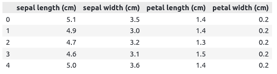
iris = datasets.load_iris()

Now, let’s print a few rows of the dataset to get familiar with the type of data.

# importing the pandas
import pandas as pd
# convertig the dataset into pandas dataframe
data = pd.DataFrame(iris.data, columns=iris.feature_names)
# head
data.head()

Output:

We can also print out the output class to see the kind of data we have in the output class.

# output class
iris.target

Output:

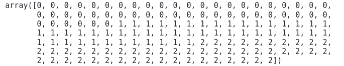
Notice that the output class contains only three categorical values.

The next step is to check if the dataset is balanced or unbalanced. We will use a pie chart to plot the output categories to see how well our dataset is balanced.

#creating variables
specie1=0
specie2 = 0
specie3 = 0
labels=["specie 1", 'specie 2', 'specie3']
# for loop to count the outputs
for i in iris.target:
    if i ==0:
        specie1+=1
    elif i ==1:
        specie2+=1
    else:
        specie3+=1
# importing required module
import matplotlib.pyplot as plt
fig = plt.figure()
# Creating plot
fig = plt.figure(figsize =(10, 7))
plt.pie([specie1, specie2, specie3], labels = labels)
 
# show plot
plt.show()

Output:

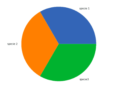
This shows that our data is perfectly balanced.

Splitting the dataset

Before training the model, we will split the dataset into training and testing part so that later we can evaluate the performance of our model.

We will store the input and output data in separate variables.

# input and output
Input, output = datasets.load_iris(return_X_y=True)

The next step is to split the dataset into the testing and training parts. We will assign 75% of the data to the training and the remaining 25% to the testing.

# importing the module
from sklearn.model_selection import train_test_split
# splitting the dataset
X_train, X_test, y_train, y_test = train_test_split(Input, output, test_size=0.25)

Once splitting is done, we can start training the model. We will train the model on a different number of stump trees and will compare the results.

Training the model on 1 stump tree

For demonstration purposes, let’s initialize the AdaBoost with only 1 stump tree.

# Import the AdaBoost classifier
from sklearn.ensemble import AdaBoostClassifier
# Create adaboost classifer with 1 stump trees
Ada_classifier = AdaBoostClassifier(n_estimators=1)

Now we will train the classifier on the training dataset.

# Train Adaboost Classifer
AdaBoost = Ada_classifier.fit(X_train, y_train)

Once the training is complete, we will use the testing data to predict the output values and store them in a variable.

#Predict the response for test dataset
AdaBoost_pred = AdaBoost.predict(X_test)

Now we have predictions of the model trained on 1 stump tree. Let’s now calculate the accuracy of the model.

# importing the module
from sklearn.metrics import accuracy_score
# printing
print("The accuracy of the model is:  ", accuracy_score(y_test, AdaBoost_pred))

Output:

This shows that 60% of the testing dataset was classified correctly by the AdaBoost algorithm when trained using only one stump tree.

Training the model on 20 stump trees

Now let’s increase the number of stump trees to 20 and see how the predictions of the model change.

# Create adaboost classifer with 20 stump trees
Ada_classifier = AdaBoostClassifier(n_estimators=20)
# Train Adaboost Classifer
AdaBoost = Ada_classifier.fit(X_train, y_train)
#Predict the response for test dataset
AdaBoost_pred = AdaBoost.predict(X_test)

Let us now find the accuracy of the model.

# printing
print("The accuracy of the model is:  ", accuracy_score(y_test, AdaBoost_pred))

Output:

This time we’ve got much better (accurate) predictions. That became possible because we’ve increased the number of stump trees to help the model to decrease the total prediction errors. But it does not means increasing the stump trees will always increase the accuracy.

Also, it is not always possible to guess with the optimum number of stump trees. However, there are various ways to find the optimum number of trees. In this article, we will be using the GridSearchCV helper class.

Using GridSearchCV to find optimum stump trees number

GridSearchCV class allows us to find the best set of parameters from the provided ranges for such parameters. Basically, it calculates the model’s performance for every single combination of provided parameters and outputs the best parameters combination.

Let’s apply the GridSearchCV to find an optimum number of stump trees for the AdaBoost algorithm:

# importing required module
from sklearn.model_selection import GridSearchCV
# initializing the model
model=AdaBoostClassifier()
# applying GridSearchCV
grid=GridSearchCV(estimator=model,param_grid={'n_estimators':range(1,50)})
# training the model
grid.fit(X_train,y_train)
# printing the best estimator
print("The best estimator returned by GridSearch CV is:", grid.best_estimator_)

Output:

This shows that the optimum number of stump trees for the Adaboost on our dataset is 5.

Let’s train the model on 5 stump trees and see the accuracy:

# Create adaboost classifer with 5 stump trees
Ada_classifier = AdaBoostClassifier(n_estimators=5)
# Train Adaboost Classifer
AdaBoost = Ada_classifier.fit(X_train, y_train)
#Predict the response for test dataset
AdaBoost_pred = AdaBoost.predict(X_test)
# printing
print("The accuracy of the model is:  ", accuracy_score(y_test, AdaBoost_pred))

Output:

We’ve got 97% accuracy for our model for this dataset using only 5 stump trees.

Implementation of AdaBoost algorithm on the regression problem

A dataset having continuous output values is known as a regression dataset. In this section, we will be using a dataset that contains information about the prices of houses in Dushanbe Tajikistan. The dataset contains the number of floors, number of rooms, area, and location of houses as independent variables and the price of the house as an output. Let’s first, explore the dataset.

Importing and exploring the dataset

We will use the pandas module to import the dataset. You can get access to the dataset using this link.

# importing the module
import pandas as pd
# importing the dataset
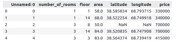
house = pd.read_csv("Dushanbe_house.csv")

Once we import the dataset, we can use head() method to print a few rows to get familiar with the dataset.

# head() method
house.head()

Output:

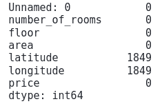
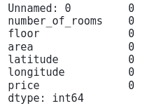
Our dataset contains null values, so we need to take care of them before using this data for training the model. Let’s use isnull() and sum() method to get the total number of null values.

# total null values
house.isnull().sum()

Output:

There’re various ways for handling dataset null values problem, but for simplicity, we’ll just drop them. Let’s use the dropna() method to do this:

# removing the null values
house = house.dropna(axis=0 , )
# null values
house.isnull().sum()

Output:

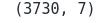
Let’s check the shape of the dataset:

# shape 
house.shape

Output:

Visualizing dataset

We will now use the plotly module to visualize the dataset to analyze how the input data is related to the price.

Let’s first see how the area of the houses affects the price of the house. We can plot the price on the y-axis and the area of the house on the x-axis:

# importing the module
import plotly.express as px
# plotting scattered plot
fig = px.scatter(y=house['price'], x = house['area'])
# fig = px.scatter(x=predictions)
fig.show()

Output:

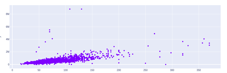
This shows that as the area of the houses increase, the price also increases with few exceptions.

Let’s now visualize the locations of these houses by plotting them using latitude and longitude.

# plotting the graph
fig = px.scatter(y=house['longitude'], x = house['latitude'])
# showing
fig.show()

Output:

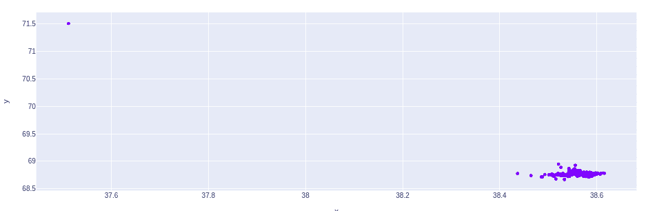
Notice that except for one house, all other houses are located near to each other.

Splitting the dataset

As we understand the dataset clearly, we can now split it into testing and training parts to that we can train the model.

# splitting dataset
x_data = house.drop('price', axis=1)
y_data = house.price

Now we can split the dataset into the testing and training parts. We will specify 70% of the data for training and 30% for the testing part.

# splitting the dataset
x_train, x_test, y_train, y_test = train_test_split(x_data, y_data, test_size = 0.3, random_state = 0)

Once the splitting is complete, we can then start training the model.

AdaBoost regressor

We can train the model using AdaBoost regressor using its default values.

# importing module
from sklearn.ensemble import AdaBoostRegressor
# Create adaboost regressor with default parameters
Ada_regressor = AdaBoostRegressor()
# Train Adaboost Classifer
AdaBoost_R = Ada_regressor.fit(x_train, y_train)

Once the training is complete, we can then predict values by passing the testing dataset.

#Predict price of houses
AdaBoostR_pred = AdaBoost_R.predict(x_test)

Let’s visualize predicted values and actual values to understand how well our model is predicting the prices of houses.

# importing the module
import matplotlib.pyplot as plt
# fitting the size of the plot
plt.figure(figsize=(20, 8))
# plotting the graphs
plt.plot([i for i in range(len(y_test))],AdaBoostR_pred, label="Predicted values")
plt.plot([i for i in range(len(y_test))],y_test, label="actual values")
plt.legend()
plt.show()

Output:

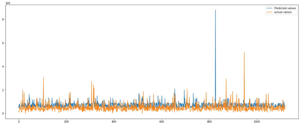
The graph shows that our predictions are a little bit lower than the actual values in most of the cases. We can evaluate the model’s performance using the R² score. The R² score is usually between one and zero. The higher the value will be, the better the model is in making predictions.

# Importing r2 
from sklearn.metrics import r2_score
# Evaluating the model
print('R-square score is :', r2_score(y_test, AdaBoostR_pred))

Output:

R²-score is negative only when the chosen model does not follow the trend of the data, which means our model was not trained properly.

GridSearchCV to find optimum stump trees

Now let’s use the GridSearchCV helper to find the optimum stump trees number.

# importing required module
from sklearn.model_selection import GridSearchCV
# initializing the model
model=AdaBoostRegressor()
# applying GridSearchCV
grid=GridSearchCV(estimator=model,param_grid={'n_estimators':range(1,50)})
# training the model
grid.fit(x_train,y_train)
# printing the best estimator
print("The best estimator returned by GridSearch CV is:", grid.best_estimator_)

Output:

This returns that the optimum number of stump trees for the given data is 4.

AdaBoost regressor using optimum stump trees

Let’s again train our model using the optimal number of stump trees which we found in the previous section of the article.

# Create adaboost regressor with default parameters
Ada_regressor4 = AdaBoostRegressor(n_estimators=4)
# Train Adaboost Classifer
AdaBoost_R4 = Ada_regressor4.fit(x_train, y_train)
#Predict price of houses
AdaBoostR_pred4 = AdaBoost_R4.predict(x_test)

We will visualize the actual and predicted values of the model again.

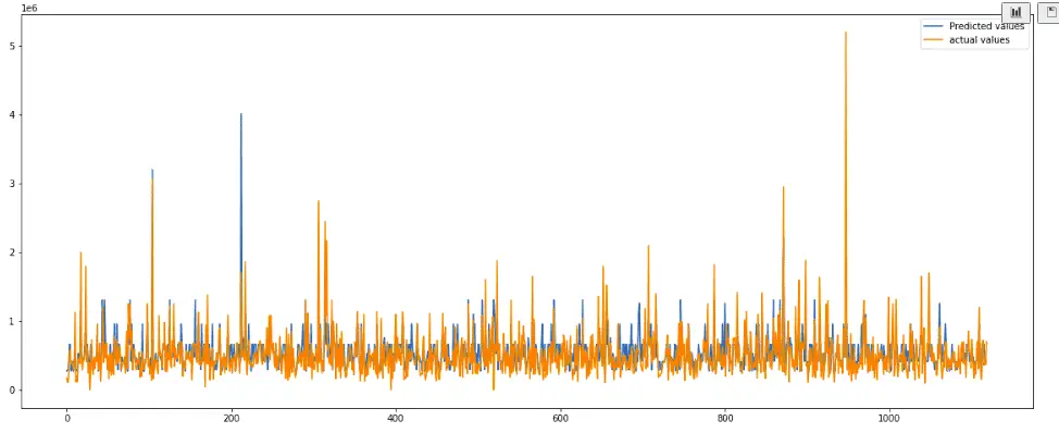
This time we can see that our model has predicted well as compared to the previous one. Let’s calculate the R²-score as well.

# Evaluating the model
print('R score is :', r2_score(y_test, AdaBoostR_pred4))

Output:

This shows that our model has performed pretty well this time.

Additional Learning Materials

From our point of view, these are the best hands-on online courses related to Machine Learning and Deep Learning available on the market right now:

Summary

AdaBoost was the first successful boosting algorithm developed for binary classification. In this article, we’ve covered the AdaBoost algorithm implementation and demonstrated how to use it to solve regression and classification problems.