Implementing KNN Algorithm using Python

KNN is a supervised, non-parametric, and lazy learning algorithm mainly used to handle classification problems. The classification problem is a problem where the output is categorical or discrete. The KNN algorithm can compete with the most accurate models because it makes highly accurate predictions. The distance measure affects the accuracy of the predictions. As a result, the KNN algorithm is appropriate for applications with significant domain knowledge. This article will cover the KNN algorithm theory, its implementation using Python, and the evaluation of the results using a confusion matrix. We will be using AWS SageMaker and Jupyter Notebook for visualization and implementation purposes.

KNN (or k-nearest neighbors) algorithm is also known as Lazy learner because it doesn’t learn a discriminative function from the training data but memorizes the training dataset instead. There is no trained model for KNN. In fact, each time we run the algorithm, it each time processes the entire model to provide the output.

KNN algorithm is non-parametric. The term non-parametric refers to the absence of any assumptions about the underlying data distribution. This will be useful in practice, as most real-world datasets do not adhere to mathematical theoretical assumptions.

Training a model using KNN algorithm

The KNN algorithm is quite accessible and easy to understand. This algorithm will look for the K number of instances defined as similar based on the nearest perimeter to a data point that isn’t in the dataset. Before feeding the data to our KNN model, we should identify if the given dataset represents a binary classification problem or a multi-class classification.

Binary classification is a classification type with only two possible output classes. For example, True or False, 0 or 1, Yes or No, and many more. In such classification, the output data set will have only two discrete values representing the two categories/classes.

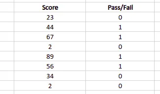
Note: that the output class contains only two discrete values, 0 and 1, representing fail and pass. There is no limit on the number of input classes. They can be up to any number depending on the complexity of the problem.

Multi-class classification is again a type of classification with more than two output classes. There will be more than two discrete values in the output in such a classification. For example classifying different animals, predicting the grades of students, and many more.

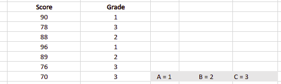
Note: that there are three different classes in the output category: 1, 2, and 3, representing grades A, B, and C, respectively. Again there is no limit on the number of input classes. Depending on the complexity of the problem, we can have as many input classes as possible.

Mathematical calculation of KNN algorithm

The concept of finding nearest neighbors may be defined as the process of finding the closest point to the input point from the given data set. The algorithm saves all available cases (test data) and categorizes new cases based on the majority votes of its K neighbors. The initial step in developing KNN is to convert data points into mathematical values. The algorithm works by finding the distance between the mathematical values of these points. It calculates the distance between each data point and the test data, then determines the probability of the points being similar to the test data.

The distance function in KNN might be the Euclidean, Minkowski, or the Hamming distance. Among which the Euclidean is the most popular and simple one. In this article, our focus will be on the Euclidean distance formula.

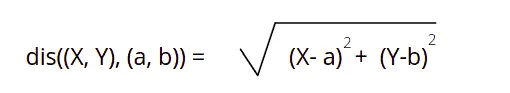
This is the simplest distance formula. It calculates the shortest distance between the two points. Graphically, it can be represented as follows:

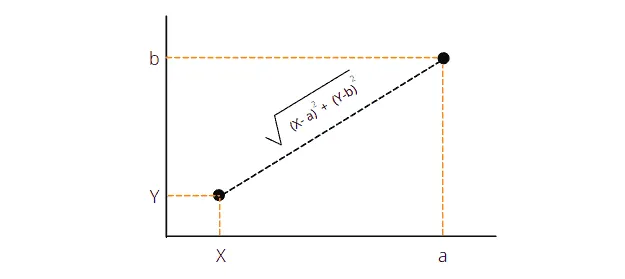
The KNN algorithm uses the distance formula to find the shortest distance between the input and training data points. It classifies the input data point. Then it selects the k-number of shortest distances based on the majority voting.

How does KNN algorithm work?

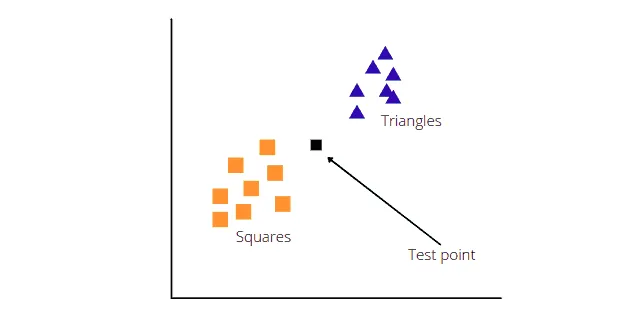
The KNN algorithm classifies the new data points based on their nearest neighbors. For example, we have a new data point, and we need to classify it using the KNN algorithm.

The KNN algorithm will now calculate the distance between the test and other data points. Then based on the K value, it will take the k-nearest neighbors. For example, let’s use K = 3.

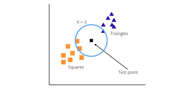
The algorithm will take three nearest neighbors (as specified K = 3) and classify the test point based on the majority voting. In our case, there were two squares and one triangle when the K = 3, which means the test point will be classified as a Square.

Python implementation of KNN algorithm

Let’s implement the KNN algorithm in Python using its various Python modules. We will use a binary dataset to train our model and test it. You can download the dataset here. The dataset contains two input classes: Age and Salary. The output (Purchases) also contains two classes, meaning this dataset represents a binary classification problem.

Prerequisites

Before implementing the Python code for the KNN algorithm, ensure that you have installed the required modules on your system. The following modules are required for the KNN algorithm’s implementation:

• pandas
• sklearn
• matplotlib

You can install the mentioned modules on your AWS SageMaker Jupyter Notebook by executing the following commands in your cell:

%pip install pandas
%pip install sklearn
%pip install matplotlib
%pip install chart_studio
%pip install plotly

Once the modules are installed, you can check the version of each one by executing the following code:

#importing the required modules
import matplotlib
import sklearn
import pandas
#printing the versions of installed modules
print("matplotlib: ", matplotlib.__version__)
print("sklearn :", sklearn.__version__)
print("pandas :", pandas.__version__)

Output:

Visualizing the data set in AWS Jupyter Notebook

KNN algorithm needs a balanced data set to make an accurate classification. A balanced dataset means there should not be too much difference between output classes. For example, if one output class contains thousands of numbers and another one may be less than a hundred, then the algorithm will be biased and unable to predict accurately. That is why it is important to have a balanced dataset.

We can verify our data’s balance by visualizing it in AWS Jupyter Notebook by using the following Python program.

# importing the required modules for data visualization
import matplotlib.pyplot as plt
import chart_studio.plotly as py
import plotly.graph_objects as go
import plotly.offline as pyoff
import pandas as pd
# importing the dats set
data = pd.read_csv('KNN_Data.csv')
# counting the total output data from purchased column
target_balance = data['Purchased'].value_counts().reset_index()
# dividing the output classes into two sections
target_class = go.Bar(
    name = 'Target Balance',
    x = ['Not-Purchased', 'Purchased'],
    y = target_balance['Purchased']
)
# ploting the output classes
fig = go.Figure(target_class)
pyoff.iplot(fig)

Output:

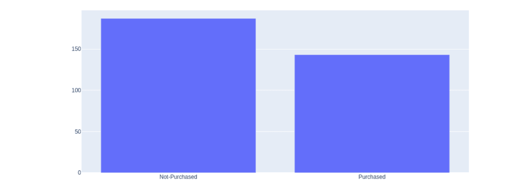
Note: the data is not unbalanced. It shows that above 180 people have not purchased the product while nearly 150 people have purchased it. That means this data is suitable for the KNN algorithm, and we can train our model using this dataset.

Implementation of KNN algorithm using Python

Let us now jump into the implementation part by importing the required modules.

# importing the required modules
import matplotlib.pyplot as plt
import pandas as pd

The pandas the module is used to import the data set and divide it into an inputs data frame and output data frame, respectively, while the Matplotlib is used to visualize the results and dataset. Let us now import the dataset and divide it into inputs and outputs.

# Import the data set for KNN algorithm
dataset = pd.read_csv('KNN_Data.csv')
# storing the input values in the X variable
X = dataset.iloc[:,[0,1]].values
# storing all the ouputs in y variable
y = dataset.iloc[:,2].values

We have imported the dataset and then stored all the data (input) except the last column to the X variable. The last column contains outputs, and we need to exclude them from the input. The data from the last column (output) is stored in the y variable.

To have the ability to test the accuracy of our model later, let’s split our data into training (70%) and testing (30%) datasets:

# importing the train_test_split method from sklearn
from sklearn.model_selection import train_test_split
# splitting the data 
X_train, X_test, y_train, y_test = train_test_split(X, y, test_size=0.30, random_state=0)

The next step is to scale the features data.

Feature scaling is a technique to standardize the independent features present in the data in a fixed range. If feature scaling is not done, a Machine Learning algorithm will assume larger values to have more weight and smaller values to have less weight, regardless of the unit of measurement.

# applying standard scale method
from sklearn.preprocessing import StandardScaler
sc = StandardScaler()
# scaling training and testing data set
X_train = sc.fit_transform(X_train)
X_test = sc.transform(X_test)

Once the data scaling is done, we can then feed the training data to the KNN algorithm to train our model.

# importing KNN algorithm
from sklearn.neighbors import KNeighborsClassifier
# K value set to be 3
classifer = KNeighborsClassifier(n_neighbors=3 )
# model training
classifer.fit(X_train,y_train)
# testing the model
y_pred= classifer.predict(X_test)

Note: we provide both the inputs and outputs of the training dataset to train the model. After the training part, we provide the inputs of the testing data and stores the predicted output in a variable y_pred. Once we have the predicted outputs, we can then check the accuracy of the trained model.

# importing accuracy_score
from sklearn.metrics import accuracy_score
# printing accuracy
print(accuracy_score(y_test,y_pred))

Output:

This shows that the accuracy of our model is 84%, which is pretty good.

How to select K value?

Instead of randomly choosing the K-value, we can use error curves to get the optimal K-value. You need to look for a function minimum for the train data.

Let’s ploterror curves:

# Importing the numpy modlule
import numpy as np
# creating sets for errors
error1= []
error2= []
# for loop 
for k in range(1,15):
    # using KNN algorithm
    knn = KNeighborsClassifier(n_neighbors=k)
    knn.fit(X_train,y_train)
    y_pred1 = knn.predict(X_train)
    # stroring the errors
    error1.append(np.mean(y_train!= y_pred1))
    y_pred2 = knn.predict(X_test)
    error2.append(np.mean(y_test != y_pred2))
# ploting the graphs for testing and training 
plt.plot(range(1,15), error1, label="train")
plt.plot(range(1,15), error2, label="test")
plt.xlabel('k Value')
plt.ylabel('Error')
plt.legend()

Output:

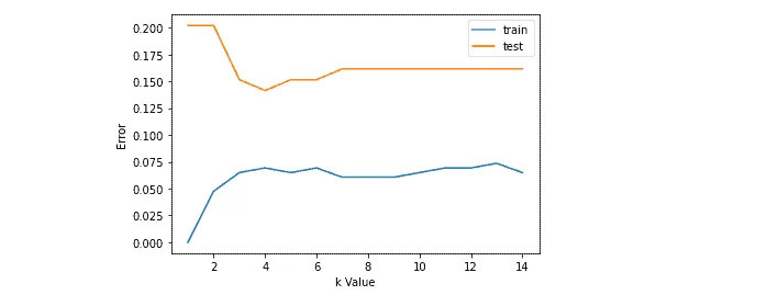
Based on the above graph, our trained model will give an optimal solution when the K = 4.

Let’s change the value of K to 4 in our model (then_neighbors variable in the classifier):

# importing KNN algorithm
from sklearn.neighbors import KNeighborsClassifier
# K value set to be 4
classifer = KNeighborsClassifier(n_neighbors=4)
# model training
classifer.fit(X_train, y_train)
# testing the model
y_pred= classifer.predict(X_test)
# importing accuracy_score
from sklearn.metrics import accuracy_score
# printing accuracy
print(accuracy_score(y_test, y_pred))

Output:

This time the accuracy has increased and given us 85.8% accurate results. But for the best practice, we should not use any even number for the K value because it can sometimes give strange results.

KNN algorithm using Python and AWS SageMaker Studio

Now let us implement the KNN algorithm using AWS SageMaker, where we are using Python version 3.7.10.

# importing the required modules
import matplotlib.pyplot as plt
import pandas as pd
# Import the data set for KNN algorithm
dataset = pd.read_csv('KNN_Data.csv')
# storing the input values in the X variable
X = dataset.iloc[:,[0,1]].values
# storing all the ouputs in y variable
y = dataset.iloc[:,2].values
# importing the train_test_split method from sklearn
from sklearn.model_selection import train_test_split
# splitting the data 
X_train, X_test, y_train, y_test =train_test_split(X,y,test_size=0.25, random_state=7)
# importing KNN algorithm
from sklearn.neighbors import KNeighborsClassifier
# K value set to be 3
classifer = KNeighborsClassifier(n_neighbors=3)
# model training
classifer.fit(X_train, y_train)
# testing the model
y_pred= classifer.predict(X_test)
# importing accuracy_score
from sklearn.metrics import accuracy_score
# printing accuracy
print(accuracy_score(y_test, y_pred))

Output:

Notice that we have changed the random state and test_size which affects our result.

Evaluating KNN algorithm performance

In this section of the article, we’ll show how to evaluate KNN algorithm performance.

Confusion Matrix

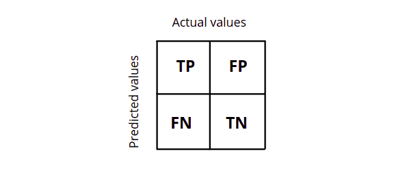
A confusion matrix is a method of summarizing a classification algorithm’s performance. It is simply a summarized table of the number of correct and incorrect predictions. Calculating a confusion matrix can give us a better idea about the miss-classified classes. We can easily determine the model’s accuracy by examining the diagonal values by visualizing the confusion matrix.

When considering the structure confusion matrix, the number of output classes is directly proportional to the size of the matrix.  It is a square matrix where the column reflects actual values and the row represents the model’s predicted value or vice versa.

What is True Postive (TP)?

A true positive is an outcome where the model correctly predicts the positive class. In simple words, the model predicts the true value. For example, If we have output classes in the training dataset; One is a cat class representing the positive class, and another is a dog class representing the negative class. And let us say the input image was a cat, and then our algorithm also classified the image as a cat, then we say it belongs to a true positive value as both the predicted and the actual value are True.

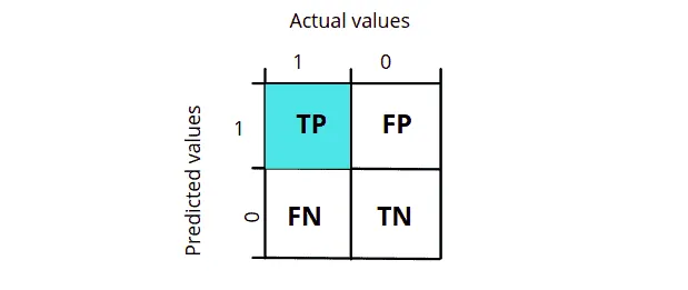
As shown in the diagram, the true positive is when the actual value is true or 1, and the model also predicts the value to be true or 1.

What is True Negative (TN)?

A true negative is an outcome where the model correctly predicts the negative class. In other words, the model correctly predicts the false value. For example, if a dog class represents a false/negative class in our training dataset and when the image of a dog is provided to model to predict and if it predicts the image as a dog, then we say it is a true negative because the model predicts the false/negative class correctly.

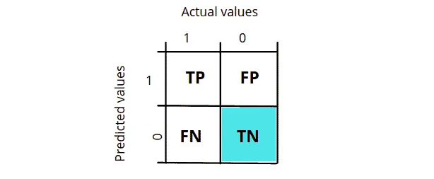
As shown in the diagram, True Negative is when the actual value is false or 0, and the model also predicts the output to be false or 0.

What is False Positive (FP)?

A false positive is an outcome where the model incorrectly predicts the positive class. In simple words, when the model predicts a value to be true, it is a false value in reality. Taking the same example of dog and cat, when our model classifies the dog image as a cat, we say it is False Positive.

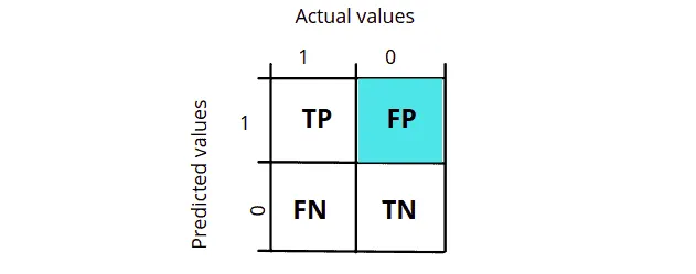
Notice that in the False positive, the actual value is false or 0, but the model predicts the output to be true or 1.

What is False Negative (FN)?

A False negative is an outcome where the model incorrectly predicts the negative class. For example, when our model classifies the image of a cat as a dog, we say it is a False Negative. In other words, when the model predicts a value to be false, it is a True value in reality.

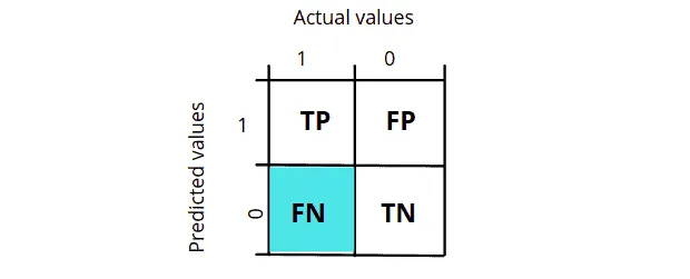
Notice that the actual value was 1, but the model predicted it to be 0 in False Negative, as shown in the diagram above.

Confusion Matrix for binary classification

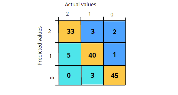
We already know that a binary classification contains two output classes. Similarly, a confusion matrix that shows the binary classification result also contains two output classes. We can calculate the precision, accuracy, recall, and F1-score by looking at the given confusion matrix. We have the following confusion matrix representing a binary classification problem and predicted outputs.

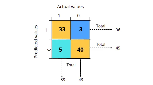
The confusion matrix above gives us much useful information. For example, we can see that 33 out of 38 true classes were classified correctly. At the same time, 5 of them were placed incorrectly, and 40 out of 43 false classes were classified correctly, while 3 of them were misclassified. Using this matrix, we can calculate the model’s accuracy, precision, recall, and f1-score. But first, let us assign the values to their respective sections.

• True Positive (TP) = 33
• True Negative (TN) = 40
• False Positive (FP) = 3
• False Negative (FN) = 5

Precision and Accuracry

In Machine learning, accuracy is the measurement to determine which model is best at identifying relationships and patterns between variables in a dataset based on the input or training data. In classification problems, accuracy helps us know how accurate our model is in classifying different classes. The following formula is used to find the accuracy of the classifying model.

In other words, accuracy is the total number of positive predictions divided by the total number. For example, in the above case, the accuracy will be (33+40)/(33+40+3+5) = 0.9 (90% of results are accurate).

Precision is another indicator of a machine learning model’s performance. It is the quality of a positive prediction made by the model. In simple words, Precision refers to the number of true positives divided by the total number of positive predictions.

The precision of the above example will be, (33)/(33+3) = 0.91.

Recall and F1-Score

The recall is the measure of our model correctly identifying True Positives. In other words, recall is the number of true predicted values divided by true predicted values and false negative values.

The recall value of our previous example will be (33)/(33+5) = 0.86.

While the F1 Score is the weighted average of Precision and Recall, this score takes both false positives and false negatives. Intuitively it is not as easy to understand as accuracy, but F1 is usually more useful than accuracy, especially if we have an uneven class distribution.

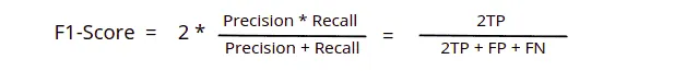
Based on the above formula. the F1-score of our example will be (2*33)/(2*33 + 3 + 5) = 0.89.

Confusion matrix for binary classification using Python

We already know how to build a confusion matrix and calculate accuracy, precision, recall, and f1-score. Let us now implement the confusion matrix using python and find out the accuracy and precision of our trained model.

# importing seaborn
import seaborn as sns
# Making the Confusion Matrix
from sklearn.metrics import confusion_matrix
# providing actual and predicted values
cm = confusion_matrix(y_test, y_pred)
# If True, write the data value in each cell
sns.heatmap(cm,annot=True)
# saving confusion matrix in png form
plt.savefig('confusion_Matrix.png')
print(cm)

Output:

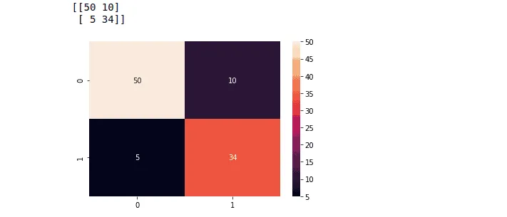
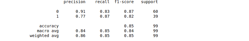
We can also find the accuracy, recall, and precision by using sklearn module to know how well our model is performing.

# importing accuracy score
from sklearn.metrics import accuracy_score
accuracy_score(y_test,y_pred)
# finding the whole report
from sklearn.metrics import classification_report
print(classification_report(y_test, y_pred))

Output:

Confusion matrix for multiclass classification

We know that multiclass classification is a classification where we have more than two output classes. The true positive values will be all the values in the diagonal of the confusion matrix.

In the case of multiclass classification, the TP, TN, FP, and FN are as follows:

• True Positive: Sum of the daigonal values
  • TP = 33 + 40 + 45
• False Positive: Sum of Values in Corresponding Column (Excluding TP).
  • FP = (5 + 0) + ( 3 + 3) + (2 + 1)
• False Negative: Sum of Values in Corresponding Row (Excluding TP).
  • FN = (3 + 2) + ( 5 + 1) + ( 0 + 3)
• True Negative: Sum of All Columns and Rows (Excluding that column’s and row).
  • TN = (40+1+3+45) + ( 5 + 1+0+45) + (5+40+0+3)

Notice that in the case of multi-class classification, the FP and FN have the same value. The precision, accuracy, recall, and f1-score use the same formulae in the case of multi-class classification.

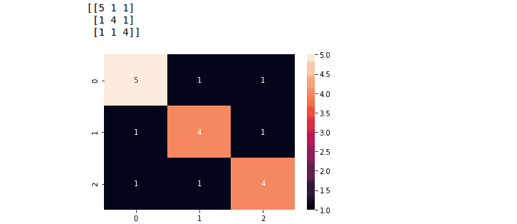
Confusion matrix for multiclass classification using Python

There is no difference in the implementation part of the code in binary and multiclass classification. The only difference is the dataset (with more than two outputs), and confusion matrix, which will have as many rows and columns as many the dataset has outputs. For the demonstration purpose, we will use sample data containing actual and predicted outputs. You can get access to the data from here.

# importing the modules
import pandas as pd
import seaborn as sns
# import the data set from Desktop
dataset = pd.read_csv('MultiClass.csv')
Actual = dataset.iloc[:,0].values
Predicted = dataset.iloc[:,1].values
# Making the Confusion Matrix
from sklearn.metrics import confusion_matrix
cm = confusion_matrix(Actual, Predicted)
# If True, write the data value in each cell
sns.heatmap(cm,annot=True)
plt.savefig('h.png')
print(cm)

Output:

Similarly, we can find the accuracy, precision, recall, and f1-score for multi-class classification the same way as we did for binary classification.

Ploting error rate in AWS SageMaker Studio

It is sometimes difficult to develop a K value that gives the lowest error and highest accuracy. However, we can plot the error rate graph for different values of K and can visually see the value of K, which gives the lowest error.

# import numpy
import numpy as np
error_rate = []
# searching k value upto  40
for i in range(1,40):
    # knn algorithm 
    knn = KNeighborsClassifier(n_neighbors=i)
    knn.fit(X_train, y_train)
    # testing the model
    pred_i = knn.predict(X_test)
    error_rate.append(np.mean(pred_i != y_test))
# Configure and plot error rate over k values
plt.figure(figsize=(10,4))
plt.plot(range(1,40), error_rate, color='blue', linestyle='dashed', marker='o', markerfacecolor='red', markersize=10)
plt.title('Error Rate vs. K-Values')
plt.xlabel('K-Values')
plt.ylabel('Error Rate')

Output:

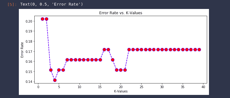
The graph above shows that the model predicts well when the value of k is 4, as we have observed before.

Summary

The K-Nearest Neighbors algorithm computes a distance value for all node pairs in the graph and creates new relationships between each node and its k-nearest neighbors. It is also a lazy learner as the model is not trained for long-term use. Each time we run the algorithm, it trains itself and computes results. It helps us calculate the trained model’s accuracy, precision, recall, and f1-score. A confusion matrix is a summary of predictions of the classification problem. The correct and incorrect predictions are totaled and broken down by class using count values. This article discussed the KNN algorithm using python in detail and covered the confusion matrix for binary and multiclass classification problems. We have used AWS Jupyter notebook and AWS SageMaker Studio to implement the KNN algorithm.