NumPy – Quick And Simple Introduction

NumPy is a library for the Python programming language, adding support for large, multidimensional arrays and matrices, along with an extensive collection of high-level mathematical functions to operate on these arrays. This article covers how to use NumPy arrays, indexing, sorting, shaping, and slicing operations. We will also cover how different NumPy methods can help preprocess data for Machine Learning algorithms.

NumPy is an open-source Python library often used with Pandas, SciPy (Scientific Python), and Matplotlib (plotting library). You can easily replace MatLab (a popular technical computing platform) with these packages. NumPy’s main object is the homogeneous multidimensional array (a list of elements of the same type indexed by a tuple of nonnegative integers).

Installing NumPy

The NumPy module is not available in the standard Python distribution, so we have to install it explicitly before using it. The most common way of installing the NumPy module is to use the pip command. If you are using the Jupyter Notebook, run the following command inside the cell to install the NumPy module:

%pip install numpy

If you are not using Jupyter notebook, you can run a similar command in your terminal:

pip install numpy

After the installation, you can check the details by using pip show command:

pip show numpy

Output:

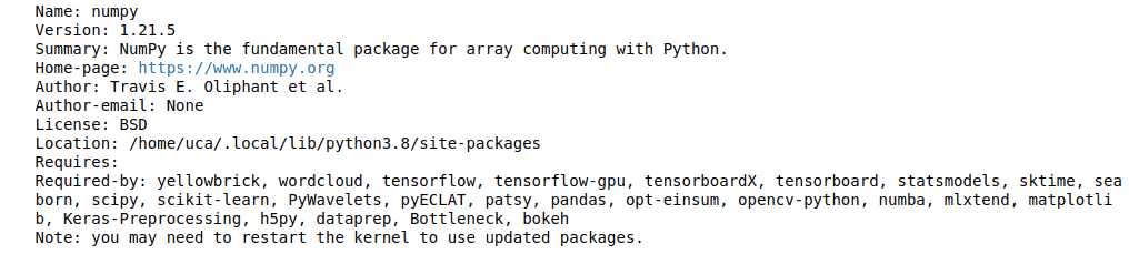
If you already have NumPy but want to upgrade it, use the following command to update the existing NumPy module to the newer version:

pip install --upgrade numpy

Now, we can import the module and start using it:

#importing NumPy module
import numpy as np

Creating NumPy arrays

A NumPy array is a data structure that consists of values of the same type indexed by a tuple of nonnegative integers.

A numpy array can be one-dimensional or multidimensional. In the upcoming section, we will discuss both array types in detail.

Now, let’s look at how to create BumPy arrays using various methods.

array()

The simplest way is to pass the Python’s list to the NumPy array() method:

# creating Python list
my_list = [1,2,3,4,5,6,7,8,9,0]
# printing the type
print(type(my_list))

Output:

Now let’s convert a regular list to a NumPy array:

# importing numpy module
import numpy as np
# converting list to numpy array
np_array = np.array(my_list)
# printing the type
print(type(np_array))

Output:

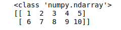
To create a multidimensional NumPy array, we need to pass a list of lists to the NumPy array() method:

# python list of lists
my_list = [[1,2,3,4,5], [6,7,8,9,10]]
# convert to NumPy array
my_array = np.array(my_list)
# printing
print(type(my_array))
print(my_array)

Output:

arange()

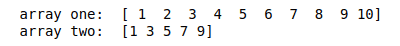
You can create a NumPy array containing a series of numbers using a built-in arange() method, which can take up to three arguments:

• starting number
• ending number
• step size

# arrange method with two agruments
my_array1 = np.arange(1, 11)
# arrange method with three arguments
my_array2 = np.arange(1, 11, 2)
# printing
print("array one: ", my_array1)
print("array two: ",my_array2)

Output:

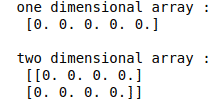
zeros()

To create a NumPy array containing filled with zero values, you can use the zeros() method and pass the number of elements:

# numpy array containing all zeros elements on dimensional
zeros1 = np.zeros(5)
#numpy array containing zeros in two dimensional
zeros2 = np.zeros((2, 4))
# printing
print("one dimensional array : \n", zeros1)
print("\ntwo dimensional array : \n", zeros2)

Output:

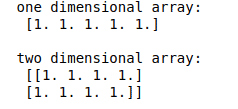
ones()

NumPy module provides another function ones() that creates an array of required sizes filled with ones:

# numpy array containing all ones in one dimensional
ones1 = np.ones(5)
# numpy array containing all ones in multi dimension
ones2 = np.ones((2, 4))
# printing
print("one dimensional array: \n", ones1)
print("\ntwo dimensional array: \n", ones2)

Output:

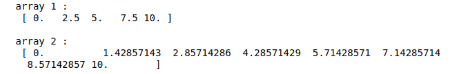
linspace()

Another powerful method to create a NumPy array is using linspace() method that produces an array of evenly spaced numbers over a specified interval. The method takes three arguments:

• beginning of the range
• end of the range
• number of points within the range

Here’s an example:

# creating numpy array using linespace
array1 = np.linspace(0, 10, 5)
array2 = np.linspace(0,10, 8)
# printing
print("array 1 :\n", array1)
print("\narray 2 :\n", array2)

Output:

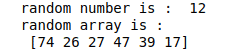
randint()

We can also use the NumPy random.randint() function to create arrays of random numbers from a specified range. If you pass only two arguments, this method will return a random number from that range. But if we specify the third argument (the size of the random array), it will return a collection of random numbers.

See the example below:

# creating random number
random_num = np.random.randint(1, 100)
# creating random array 
random_array = np.random.randint(1, 100, 6)
# printing
print("random number is : ", random_num)
print("random array is : \n", random_array)

Output:

empty()

The empty() method in the NumPy module is used to create an empty array of the specified size.

Here’s an example:

# creating emtpy array of interger numbers
array1 = np.empty([2, 3], dtype = int)
# creating empty array of floating numbers
array2 = np.empty([2, 3], dtype = float)
# printing
print("Emtpy integer type array\n",array1)
print("\nEmpty  float type array \n",array2)

Output:

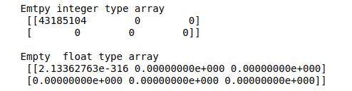
The values in the empty array are random uninitialized values.

Visualazing NumPy arrays

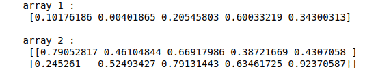
The random.rand() method is one of the most valuable methods to create a NumPy array of uniformly distributed random numbers. This method can take up to two arguments to create an array of uniformly distributed elements between 0 and 1:

# creating array of random numbers between [0, 1)
array1 = np.random.rand(5)
array2 = np.random.rand(2,5)
# printing
print("array 1 :\n", array1)
print("\narray 2 :\n", array2)

Output:

Let’s create an array of 500 elements and visualize its values using a bar chart. We will use the Plotly library for the visualization.

# creating numpy array of uniformly distribution
array1 = np.random.rand(500)
# importin the plotly module
import plotly.express as px
# creating bar chart
fig = px.bar(array1)
fig.show()

Output:

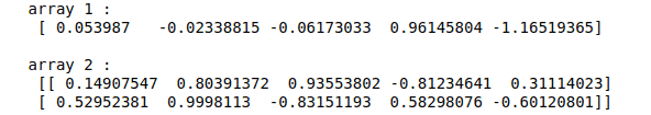
If we want to have an array of random elements from a standard normal distribution, you can use the random.randn():

# creating one dimensional array
array1 = np.random.randn(5)
array2 = np.random.randn(2, 5)
# printing
print("array 1 :\n", array1)
print("\narray 2 :\n", array2)

Output:

Now let’s visualize to see the random array elements from a standard normal distribution:

# creating an array 
array = np.random.randn(500)
# ploting using plotly
fig = px.bar(array)
fig.show()

Output:

The linspace() method creates an array of elements having the same difference between each other.

Let’s create an array using linspace() method and visualize it.

# creating an array
array = np.linspace(1, 10, 100)
# ploting the array
fig = px.bar(array)
fig.show()

Output:

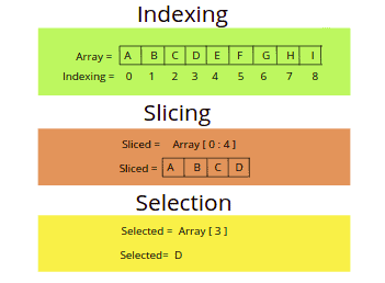
NumPy array indexing, slicing and selecting elements

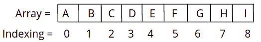
Array indexing allows you to refer to the individual array items by the element index number. The list (array) indexing in Python always starts from 0. The first element in the array will have an index of 0, the second will be 1, and so on. This section of the article will describe the list (array) and indexes for slicing and selecting elements.

Indexing and selecting elements from one dimensional array

Let’s take a look at how the NumPy array is indexed. First, we need to create an array:

# creating one-D numpy array
array = np.arange(3, 15)
# printing
print(array)

Output:

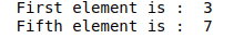
Now, we can use indexing to get access to the specific element of the NumPy array. For example, we will print the first and the fifth element of the given array:

# Accessing the elements
first_element = array[0]
fifth_element = array[4]
# printing
print("First element is : ", first_element)
print("Fifth element is : ", fifth_element)

Output:

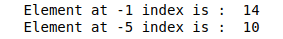
Another way to access the element is using negative indexes. The -1 value represents the index value of the last element of the array, and -2 represents the index value of the second element from the end of the array.

The following Python code accesses the elements of the array using a negative index:

# Accessing the elements with negative indexiing
one_element = array[-1]
five_element = array[-5]
# printing
print( "Element at -1 index is : ", one_element)
print("Element at -5 index is : ", five_element)

Output:

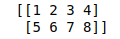
Indexing and selecting elements from n-dimensional array

Let’s take a look at how we can use indexes to access the elements from an n-dimensional array (for example, 2×4 array):

# list 
list_1 = [[1,2,3,4],[5,6,7,8]]
# numpy array
array = np.array(list_1)
# printing
print(array)

Output:

For the n-dimensional array, we have to use two indexes to access the specific element. We have to provide the index of the row and then the index value of the column.

There are two ways to do it:

• double square brackets
• single square bracket

For example, to get access to the element with value 5 (the second row and the first column) from the above array, you need to use [1][0] index defined in double square brackets.

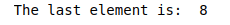
Let us now take an example and print the last element from the array:

# indexing in the n-dimensional array
last_element = array[1][3]
# printing
print('The last element is: ', last_element)

Output:

Similarly, we can also use negative indexes to access elements in the n-dimensional array. The index value -1 represents the last element in a row or column.

For example, we can select the last element by just passing the -1 value:

# negative indexing in the n-dimensional array
last_element = array[-1][-1]
# printing
print('The last element is: ', last_element)

Output:

We can use the single brackets expression to access the n-dimensional NumPy array element. Just provide the rows index and column index values separated by a comma inside the square brackets:

# using single brackets
value = array[1,1]
# printing
print(value)

Output:

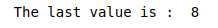
Similarly, we can use negative indexing with single brackets to select a specific value from the n-dimensional array. For example, we can choose the last value using a negative index:

# negative indexing
last_value = array[-1, -1]
# printing
print("The last value is : ", last_value)

Output:

Slicing one-dimensional NumPy array

Array slicing allows you to get a set of elements from an array by using a range index values expression:

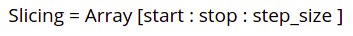
The default value for the starting index is 0, the ending index is -1, and the step size is 1.

Now, let’s create an array and use the slicing technique to slice an array:

# creating array
array = np.arange(1, 15)
# printing the array
print(array)

Output:

To get the slice of the first five elements, we need to set the start index to 0 and then stop index to the 5th index as shown below:

# slicing by the start and stop points
sliced1 = array[0 : 5]
# slicing by the stop point only
sliced2 = array[ : 5]
print("slice 1 : ", sliced1)
print("slice 2 : ", sliced2)

Output:

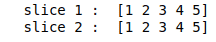
Notice that both the slices are the same because when we do not specify the starting point (by default, its value is zero).

Now let’s slice the array starting from index 5 till index 11. In this case, the starting point will be 5, and the ending point will be 11. The index 11 is not included in the sliced part as it is a stopping point.

# slice of array
slice3 = array[5 : 11]
# print
print("Slice is : ", slice3)

Output:

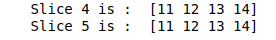
There are two ways to get a slice of all the elements starting from index 10 till the end. We can either specify the ending point or leave it blank because, by default, it will be considered the end of the array.

# slicing by the start and stop points
slice4 = array[10: 15]
# slicing by the stop point only
slice5 = array[10: ]
# printing 
print("Slice 4 is : ",slice4 )
print("Slice 5 is : ",slice5 )

Output:

We can also specify the step size for the sliced array. For example, let’s specify the step size to be 2 and print out the slice which starts from 0 and ends at 11,

# slice without step size
sliced1 = array[0 : 11]
# slice with step size
sliced2 = array[0 : 11 : 2]
# printing
print("sliced array without step size : ", sliced1)
print("sliced array with step size : ", sliced2)

Output:

If we do not specify starting, ending, and step size, we will get the same array.

# slice 
sliced = array[ : : ]
# printing
print(sliced)

Output:

One use-cases of slicing is that we can get access to the set of elements in a specified range in an array. For example, we can store 100 in the first five values using slicing as shown below:

# printing the original array
print("Original array : ", array)
# stroing value
array[0: 5] = 100
# printing
print("After stroing  : ", array)

Output:

Slicing n-dimensional NumPy array

In the same way, as we did for slicing a one-dimensional array, we can cut the n-dimensional array. But for an n-dimensional array, we have to slice the row and column simultaneously. Let’s create an n-dimensional NumPy array and then slice it.

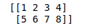
# creating 2d array
array_2d = np.array([[1, 2, 3, 4], [5, 6, 7, 8]])
# print
print(array_2d)

Output:

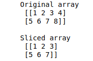
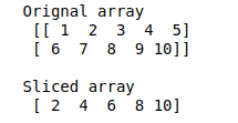
Let’s now use the indexing method to slice the NumPy array and drop the last column:

# slicing array
sliced = array[ :3 , 0:3]
# printing the original
print("Original array \n", array_2d)
# printing sliced
print("\nSliced array\n",sliced)

Output:

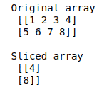
Similarly, we can use negative indexing to slice the n-dimensional array. For example, we can select the last column using negative indexing:

# slicing using negative indexing
last_column = array[:, -1:]
# printing the original array
print("Original array \n", array_2d)
# printing the sliced
print("\nSliced array\n", last_column)

Output:

Conditional selection in NumPy array

NumPy arrays allow you to select an array of elements using different conditions. For example, let’s take a look at how to get all array elements greater than 5.

# creating 1-d array
array_1d = np.array([5, 6, 7, 8, 4,10 , 5, 7, 3, 2])
# condition
array_1d > 5

Output:

The output returns an array of boolean values where:

• True – the condition is satisfied
• False – the condition is not satisfied

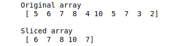
Let’s now use this condition for the array slicing:

# conditional selection
Condition = array_1d[array_1d >5]
# printing the original array
print("Original array\n", array_1d)
# printing the sliced array
print("\nSliced array\n", Condition)

Output:

Similarly, you can apply conditional selection on the n-dimensional arrays as well:

# creating n-d array
array_2d = np.array([[1, 2, 3, 4, 5], [6, 7,8, 9,10]])
# selecting 
even = array_2d[array_2d%2 == 0]
# printing original array
print("Orignal array\n", array_2d)
# printing sliced
print("\nSliced array\n", even)

Output:

Notice that the conditional sliced array is no more a 2-D array.

NumPy array operations

You can perform various operations on the NumPy array, including binary operations, arithmetic operations, some statistical and string operations. This section will cover different functions on the NumPy array by taking various examples. Let us start with binary operations.

Binary operations

Binary operators act on bits and perform the bit-by-bit operations. A binary operation is simply a rule for combining two values to create a new value.

The bitwise_and() is a NumPy built-in function used to compute the bitwise AND of two arrays element-wise. The bitwise AND operator ( & ) compares each bit of the first operand to the corresponding bit of the second operand. If both bits are 1, the corresponding bit is set to 1. Otherwise, the corresponding result bit is set to 0. Both operands to the bitwise AND operator must have integral types.

Let’s take an example to understand the working of the bitwise AND operator on the NumPy array:

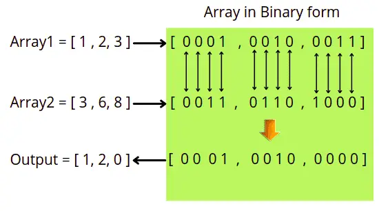
# creating np array
array1 = np.array([1, 2, 3])
array2 = np.array([3,6, 8])
# bitwise AND operation
output_array = np.bitwise_and(array1, array2)
# printing
print(output_array)

Output:

You might think the output is unexpected. But it is not. The bitwise AND operation compare the bits of each number. If the corresponding bits are 1, the output is one otherwise the output is zero. For example, the binary form of 3 is 11 or 0011, and the binary form of 8 is 1000, so when we apply the bitwise AND operation, we will get 0000.

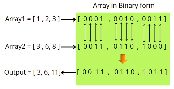
The bitwise_or() function computes the bitwise OR of two arrays element-wise. A bitwise OR is a binary operation that takes two-bit patterns of equal length and performs the logical inclusive OR operation on each pair of corresponding bits. The result in each position is 0 if both bits are 0, while otherwise, the result is 1.

Let’s apply the binary OR operation on the NumPy array:

# bitwise OR operation
output_array = np.bitwise_or(array1, array2)
# printing
print(output_array)

Output:

The OR operation works in the following way in the NumPy array.

Some other useful binary operations that you can apply on the NumPy array are:

• bitwise_xor() – computes the bit-wise XOR of two arrays element-wise.
• left_shift() – shifts the bits of an integer to the left.
• right_shift() – shifts the bits of an integer to the right.
• binary_repr() – represents binary form of the input number as a string.
• invert() – computes bit-wise inversion, or bit-wise NOT, element-wise.
• packbits() – packs the elements of a binary-valued array into bits in a uint8 array.

Arithmetic operations

Arithmetic operations are possible only if NumPy arrays have the same structure and dimensions. An arithmetic operator is a mathematical function that takes two operands and calculates them. Down below we will perform various arithmetic operations on the NumPy arrays.

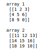
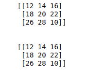
For example, we have the following NumPy array, and we need to apply various arithmetic operations:

# creating np.array
array1 = np.array([[1, 2, 3], [4, 5, 6], [8,9,0]])
array2 = np.array([[11, 12, 13], [14, 15, 16], [18,19,10]])
print("array 1 \n", array1)
print("\narray 2 \n", array2)

Output:

The two most common methods of addition of NumPy arrays are:

• addition operation +
• NumPy’s build-in method np.add()

# additing array using operator
sum1 = array1+ array2
# adding array using numpy function
sum2 = np.add(array1, array2)
# printing
print(sum1)
print(sum2)

Output:

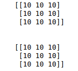
Similarly, we can apply the subtraction operation either by using the subtraction operator - or the NumPy’s built-in function np.subtract():

# subtraction using operator
sub1 = array2-array1
# subtraction using numpy function
sub2 = np.subtract(array2, array1)
# printing
print(sub1)
print("\n")
print(sub2)

Output:

Some other useful arithmetic operations available in the NumPy array are:

• divide() – returns the division of the elements.
• multiply() – return the multipication the elements
• reciprocal() – returns the reciprocal of the elements of the NumPy array.
• power() – treats elements in the first input array as base and returns it raised to the power of the corresponding element in the second input array.
• mod() – returns the remainder of division of the corresponding elements in the input array.
• real() – returns the real part of the complex data type argument.
• imag() – returns the imaginary part of the complex data type argument.

Mathematical functions

NumPy contains a large number of various mathematical operations, which include standard trigonometric functions, functions for arithmetic operations, handling complex numbers, and many more, We will discuss some of those functions in this section.

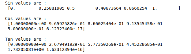
Let’s find the elements’ sin, cosine, and tangent values in an array. NumPy has built-in methods for these trigonometric functions:

# creating numpy array
array = np.array([0, 15, 30, 24, 60, 90])

# sin function 
sin = np.sin(array*np.pi/180)
# cose function
cos = np.cos(array*np.pi/180)
# tan function
tan = np.tan(array*np.pi/180)

# printing
print("Sin values are :\n", sin)
print("\nCos values are :\n", cos)
print("\nTan values are :\n", tan)

Output:

In a similar way, arcsin(), arccos(), and arctan() functions return the trigonometric inverse of sin, cos, and tan of the given angle.

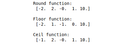
Apart from trigonometric functions, there are many other mathematical functions available. For example, around(), which returns the value rounded to the desired precision, floor() which returns the largest integer not greater than the input parameter, and ceil() which returns the ceiling of an input value.

# creating an array
array = np.array([-1.7, 1.5, -0.2, 0.6, 10])
# round method
Round = np.around(array)
# floor function
Floor = np.floor(array)
# ceil function
Ceil = np.ceil(array)
# printing
print("Round function:\n", Round)
print("\nFloor function:\n", Floor)
print("\nCeil function: \n", Ceil)

Output:

Statistical functions

NumPy has handy statistical functions for finding minimum, maximum, percentile standard deviation, and variance from the given elements in the array. These functions are primarily used in the data preprocessing and validation parts of Machine Learning.

Let’s imagine we have the following NumPy array on which we need to apply different statistical functions:

# np array
array = np.array([[1, 2, 3, 4], [5, 6, 4, 2], [9, 7, 6, 5], [1, 2, 3, 2]])
# printing
print(array)

Output:

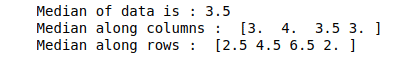
For example, the median() function returns the median. The median is the value separating the higher half of a data sample from the lower half.

# applying medin function
median = np.median(array)
median_x = np.median(array, axis=0)
median_y = np.median(array, axis=1)
# printing on of whole dat
print("Median of data is :", median)
# printing of median along x =0
print("Median along columns : ", median_x)
# printing of median along x = 1
print("Median along rows : ", median_y)

Output:

The mean() function returns the mean of the NumPy array as shown below:

# applying mean function
mean = np.mean(array)
mean_x = np.mean(array, axis = 0)
mean_y = np.mean(array, axis = 1)
# printing mean of whole data
print("Mean of data is :", mean)
# printing of mean along x =0
print("Mean along columns : ", mean_x)
# printing of mean along x = 1
print("Mean along rows : ", mean_y)

Output:

NumPy also has a built-in method for standard deviation and variance. Standard deviation is the square root of the average squared deviations from the mean, and variance is the average. Let us now calculate the standard deviation and variance of the NumPy array.

# applying standard deviation
std = np.std(array)
# applyging variance
variance = np.var(array)
# printing
print("Standard deviation is:  ", std )
print("Variance is :  ", variance)

Output:

String functions

In Python, strings are arrays of bytes representing Unicode characters. Anything written inside single or double brackets will be considered a string in Python. NumPy module provides various methods to perform different operations on Python strings, some of which we will discuss in this section.

For example the char.add() method concatenates the strings together as shown below:

# creating strings
string1 = "Wellcome to "
string2 = "hands-on-cloud!"
# adding strings using np method
added_string = np.char.add(string1, string2)
# printing
print(added_string)

Output:

The char.multiply() method returns the multiple copies of the specified string.

# string
string1 = "hands-on-cloud "
# string multipication
multiply_string = np.char.multiply(string1, 4)
# print
print(multiply_string)

Output:

The char.split() returns a NumPy array of words in the string as shown below:

# string 
string1 = 'welcome to hands on cloud'
# spliting into np array
splitted = np.char.split(string1, " ")
# printing
print(splitted)

Output:

The other common strings methods available in the NumPy module are as follows:

• char.center() – returns the copy of the string where the original string is centered with the left and right padding filled with the specified number of fill characters.
• char.capitalize() – returns a copy of the original string in which the first letter of the original string is converted to the Upper Case
• char.title() – returns the title cased version of the string.
• char.lower() – returns a copy of the string in which all the letters are converted into the lower case.
• char.upper() – It returns a copy of the string in which all the letters are converted into the upper case.
• char.splitlines() – It returns the list of lines in the string, breaking at line boundaries.
• char.strip() – returns a copy of the string with the leading and trailing white spaces removed.
• char.join() – returns a string which is the concatenation of all the strings specified in the given sequence.
• char.replace() – returns a copy of the string by replacing all occurrences of a particular substring with the specified one

Sorting and searching functions

Sorting is about putting a list/array of values in order, and searching is the process of finding the position of a value within a list/array. NumPy provides various methods for sorting and searching elements in the NumPy array.

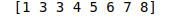
A variety of sorting-related functions are available in NumPy. For example, the sort() method returns a sorted copy of an array. By default, it uses quicksort – an algorithm for sorting elements.

# np array
array = np.array([5,4, 6, 3, 1, 7, 8, 3])
# sorting array
sorted_array = np.sort(array)
# printing
print(sorted_array)

Output:

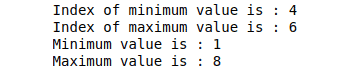
The argmax() and argmin() returns the index value of the maximum and minimum value from the array.

# np array
array = np.array([5,4, 6, 3, 1, 7, 8, 3])
# min index value
mini_index = np.argmin(array)
# max index value
max_index = np.argmax(array)
# mini value
mini_value = array[mini_index]
# max value 
max_value = array[max_index]
# printing
print("Index of minimum value is :", mini_index)
print("Index of maximum value is :", max_index)
print("Minimum value is :", mini_value)
print("Maximum value is :", max_value)

Output:

There are other various methods available in NumPy for sorting and searching, about which you can read from the NumPy Offical documentation about sorting and searching.

NumPy array shape manipulation

Shape manipulation is a technique by which we can manipulate the shape of a NumPy array and then convert the initial array into an array or matrix of the required shape and size. This may include converting a one-dimensional array into a matrix and vice-versa and finding the transpose of the matrix by using different functions of the NumPy module.

Reshaping

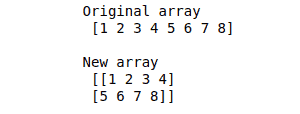
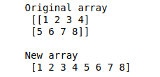
The reshape() method gives a new shape to an array without changing its data. Let’s take a one-dimensional array and convert it to ndarray using reshape method.

# creating one-d array
array_1d = np.array([1, 2, 3, 4, 5, 6, 7, 8])
# giving new shape
array_nd = np.reshape( array_1d, (2, 4))
# printing
print("Original array\n", array_1d)
print("\nNew array \n", array_nd)

Output:

Another way to modify the shape of NumPy arrays is to use the shape() method which will directly modify the shape of an array without copying it.

# convertig the shape of array
array_1d.shape = (2, 4)
# printing
print("\nNew array \n", array_1d)

Output:

In a similar NumPy has a built-in method ravel() which converts ndarray to the one-dimensional array.

# converting the array to 1d
array_1d = array_nd.ravel()
# printing
# printing
print("Original array\n", array_nd)
print("\nNew array \n", array_1d)

Output:

Stacking and joining

Stacking is the concept of joining arrays in NumPy. Arrays having the same dimensions can be stacked along a new axis. Numpy provides various methods to join arrays.

Let’s imagine we have the following two NumPy arrays:

# creating np array
array1 = np.array([[1, 2, 3], [4, 5, 6]])
array2 = np.array([[10, 22, 33], [44, 55, 66]])

The concatenate() function joins the arrays along the new axis:

# concatenating the arrays
concat = np.concatenate((array1, array2))
# printing
print(concat)

Output:

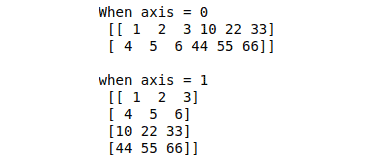
Another way to join NumPy arrays is to use append() method, which creates a new array along a specified axis.

# append method axis =0
append_y = np.append(array1, array2, axis= 0)
# append method axis =1
append_x = np.append(array1, array2, axis = 1)
print("When axis = 0\n", append_x)
print("\nwhen axis = 1\n", append_y)

Output:

You can also apply other methods to concatenate arrays discussed in the official documentation of NumPy about shape manipulation.

Summary

NumPy is a Python library consisting of multidimensional array objects and a collection of routines for processing those arrays. It is used to apply various mathematical and logical operations on arrays. This article covered how to use NumPy arrays, indexing, sorting, shaping, and slicing operations. We will also covered how different NumPy methods can help preprocess data for Machine Learning algorithms.