Python Linear Regression – Simple Tutorial

Linear Regression is one of the easiest and most popular Supervised Machine Learning algorithms. It is a technique for predicting a target value using independent factors.Linear Regression is mostly used for forecasting and determining cause-and-effect relationships among variables. This article covers the implementation of the Linear Regression algorithm using Python language. In addition, we will describe how to implement the Python Linear Regression algorithm. We will use AWS SageMaker Studio and AWS Jupyter Notebook for the implementation and visualization.

As discussed in the Overview of Supervised Machine Learning Algorithms article, Linear Regression is a supervised machine learning algorithm that trains the model from data having independent(s) and dependent variables. Based on the number of independent variables, a linear regression can be divided into two main categories:

• Simple Linear Regression: In simple Linear regression, there is only one dependent and one corresponding independent variable. That means there is only one possible output Y for every input variable X.
• Multiple Linear Regression: There are multiple independent variables and one corresponding dependent variable in multiple linear regression. That means for every output variable Y, there is more than one input variable Xi.

Best Machine Learning Books for Beginners and Experts

As Machine Learning becomes more and more widespread, both beginners and experts need to stay up to date on the latest advancements. For beginners, check out the best Machine Learning books that can help to get a solid understanding of the basics. For experts, reading these books can help to keep pace with the ever-changing landscape. In either case, a few key reasons for checking out these books can be beneficial.

First, they provide a comprehensive overview of the subject matter, mainly about Machine Learning algorithms. Second, they offer insights from leading experts in the field. And third, they offer concrete advice on how to apply Machine Learning concepts in real-world scenarios. As Machine Learning continues to evolve, there’s no doubt that these books will continue to be essential resources for anyone with prior knowledge looking to stay ahead of the curve.

Training the model in Linear Regression Algorithm

The linear Regression algorithm performs better when there is a continuous relationship between the inputs and output. We suggest you always analyze the data before applying a linear regression algorithm. You can visualize the data to see the input and output variables relationship. If the graph is scattered and shows no relationship, it is recommended not to use a Linear Regression algorithm.

For example, we have a linear dataset with one input and the corresponding output. You can download the dataset from here. Now let us visualize this dataset in AWS Sagemaker Jyputer Notebook.

# Importing the modules
import pandas as pd
import matplotlib.pyplot as plt
# Importing the dataset
dataset = pd.read_csv('DataForLR.csv')
#get a copy of dataset exclude last column
Input = dataset.iloc[:, :-1].values 
#get array of dataset in column 2st
output = dataset.iloc[:, 1].values 
# visualization part 
viz_train = plt
# applying scttered graph
viz_train.scatter(Input, output, color='blue')
viz_train.title('Hours vs Score')
# X label and Y label
viz_train.xlabel('Hours')
viz_train.ylabel('Score')
# showing the graph
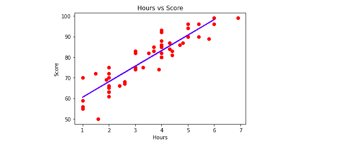
viz_train.show()

The output:

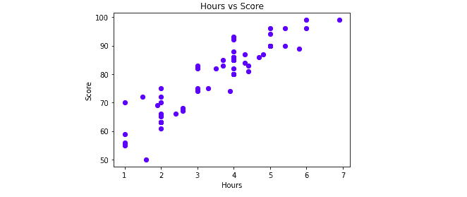
The graph shows a linear relationship between the input and output variable which means this data can be used to train the Linear Regression algorithm.

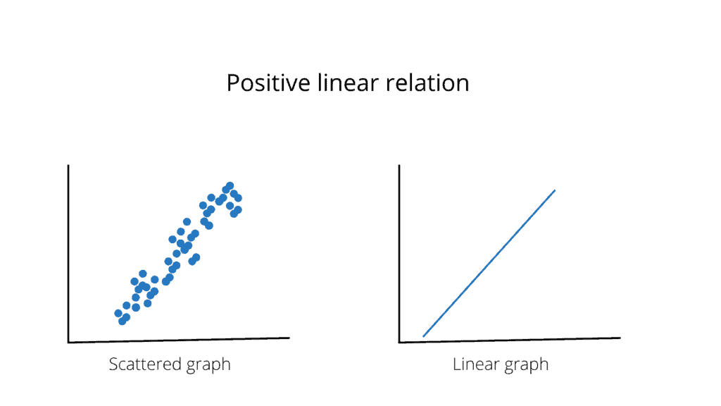
Positive Linear Relationship

A positive linear relationship is when the dependent variable expands on the Y-axis while the independent variable increases on the X-axis. In simple words, as the input variables increases, the output variables also increases. The slope of such a linear relationship will be positive.

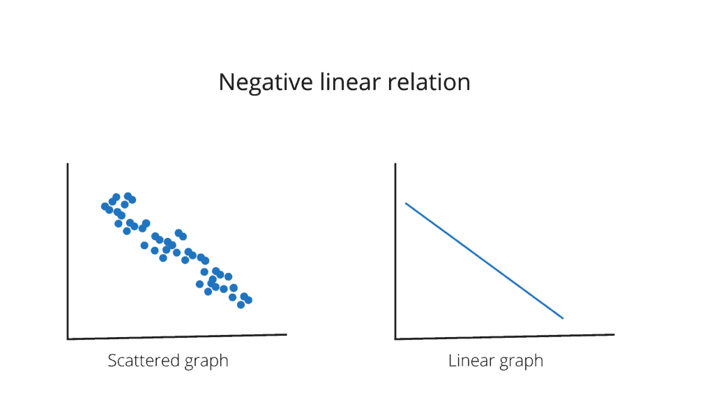
Negative Linear Relationship

A negative linear relationship is when the dependent variable decreases on the Y-axis while the independent variable increases on the X-axis. In simple words, as the input variables increases, the output variables decrease. The slope of such a linear relationship will be negative.

Mathematical calculation of training model

The Linear Regression model provides a sloped straight line representing the relationship between the variables. The following is the simple training model of Linear Regression:

• f(x) – The output of the dataset
• M – Constant value
• C – The slope of the dataset
• x – The input value of the dataset

The Linear Regression algorithm will take the labeled training data set and calculate the value of M and C. Once the model finds the accurate values of M and C, then it is said to be a trained model. Then it can take any value of x to give us the predicted output.

Implementing Python Linear Regression

This article will use Python 3.8.13 version 3.7.10 in AWS Sagemaker Jypyter Notebook, respectively. You can check the Python version running from your Jupyter Notebook notebook by executing the following code in the cell:

#importing the required module
from platform import python_version
# printing the verison
print(python_version())

This will print out the Python version on your Jypyter Notebook or SageMaker studio.

Setting up the environment

Before writing the Python program for the Linear Regression algorithm, ensure that you have installed the required Python modules. We will be using the following Python modules in this article to import the data set and train our model:

• sklearn (v0.24.2)
• pandas (v1.1.5)
• matplotlib (v3.3.4)

Use the following command to install the required modules on AWS Jupyter Notebook and SageMaker Studio:

%pip install sklearn
%pip install matplotlib
%pip install pandas

Once the modules are installed successfully, you can check the versions by typing the following Python code.

#importing the required modules
import matplotlib
import sklearn
import pandas
#printing the versions of installed modules
print("matplotlib: ", matplotlib.__version__)
print("sklearn :", sklearn.__version__)
print("pandas :", pandas.__version__)

Implementation of Linear Regression in Python

As we have installed all the required modules for the Linear Regression, we have to import them. Let us jump into the Python program and train our model using the above-mentioned dataset.

# Importing the required modules for
# Linear Regression using Python
import matplotlib.pyplot as plt
import pandas as pd

The matplotlib is used to visualize the training and testing dataset. The pandas module Is used to import the dataset and divide the dataset into input variables and output variables.

The second step is to import the dataset and split it into input and output variables using the pandas module.

# Importing the dataset
dataset = pd.read_csv('DataForLR.csv')
#get a copy of dataset exclude last column
Input = dataset.iloc[:, :-1].values 
#get array of dataset in column 2st
output = dataset.iloc[:, 1].values 

If we look back at our dataset, it has only two columns, one input column named hours, and the second is an output column named score. So, in the above program, we assign all the rows and columns, excluding the last column, to a variable named Input and assign all the rows and only the last column to the output variable.

Now the Input variable contains all the independent values, and the output variable contains the dependent values. The next step is to divide the dependent and independent classes into the training and testing data parts.

# Splitting the dataset into the Training data set and Testing data set
from sklearn.model_selection import train_test_split
# 30% data for testing, random state 1
X_train, X_test, y_train, y_test = train_test_split(Input, output, train_size=.7, random_state=1)

This is an important part of the implementation because we have split our original dataset into a training and testing dataset.

First, we have imported the training_test_split() method from the sklearn module, which splits the data set. We have specified four parameters which are:

• Input: This provides all the independent values to the function.
• output: This provides all the corresponding output values to the function.
• train_size: This is where the actual splitting of the dataset occurs. 0.7 means we have specified 70% of the dataset for the training and the remaining 30% for the testing. We can change the train_size, depending on the performance of our model.
• random: Splitting the data set into training and test parts will be random. We can assign any positive integer value. The same integer value will return the same random testing and training dataset each time we run the algorithm.

The X_train and y_train contain 70% of the original dataset, and we will use them for training our model. While X_test and y_test contain the remaining 30% of the original dataset and we will use them to test our model to see if the predictions are accurate.

We can verify the splitting of the original dataset by printing either the training part or the testing part, as shown below:

# Splitting the dataset into the Training data set and Testing data set
from sklearn.model_selection import train_test_split
# 30% data for testing, random state 1
X_train, X_test, y_train, y_test = train_test_split(Input, output, train_size=.7, random_state=1)
#printing the splitted output values
print("training output values: \n",y_train)
print("Testing output values:\n",y_test)

Output:

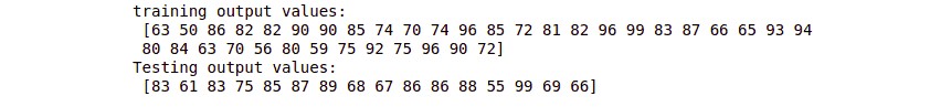
Notice that 70% of the data is in the training part, and 30% is in the testing part. Once we have successfully split the dataset, the next step is to train the model by feeding the training dataset.

# Importing linear regression form sklear
from sklearn.linear_model import LinearRegression
# initializing the algorithm
regressor = LinearRegression()
# Fitting Simple Linear Regression to the Training set
regressor.fit(X_train, y_train)
# Predicting the Test set results
y_pred = regressor.predict(X_test)

This is where the training of our model takes place. First, we initialize the linear regression algorithm and then provide the dependent and corresponding independent training dataset to train our model. Then we tested our model by only providing the independent testing dataset to our train model and saving the predicted output in a variable known as y_pred.

Visualizing the results

Our model is trained, and providing any testing value will give us the predicted output.

# Predicting single value
Pred_Salary= regressor.predict([[3]])
print(Pred_Salary)

Output:

Students who study for 3 hours will get a 75,5 score. Now, let us visualize the training dataset and the trained model. It is not an actual value but a predicted value that our trained model has predicted.

# Visualizing the Training set results
viz_train = plt
# ploting the training dataset in scattered graph
viz_train.scatter(X_train, y_train, color='red')
# ploting the testing dataset in line line
viz_train.plot(X_train, regressor.predict(X_train), color='blue')
viz_train.title('Hours vs Score')
# labeling the input and outputs
viz_train.xlabel('Hours')
viz_train.ylabel('Score')
# showing the graph
viz_train.show()

Output:

The scattered points show the actual values of the training dataset, and the blue line shows our model trained on the scattered points.

Now, let us provide the testing dataset to our model and visualize the predicted values. We will visualize the testing data using a scattered graph and a line’s predicted output.

# Visualizing the Test set results
viz_test = plt
# red dot colors for actual values
viz_test.scatter(X_test, y_test, color='red')
# Blue line for the predicted values
viz_test.plot(X_test, regressor.predict(X_test), color='blue')
# defining the title
viz_test.title('Hours vs Score')
# x lable
viz_test.xlabel('Hours')
# y label
viz_test.ylabel('Score')
# showing the graph
viz_test.show()

Output:

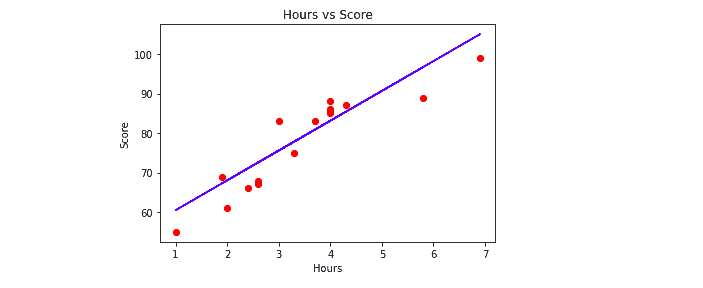
In this article, we took a sample and small data set to understand the working and implementation of Linear regression. The red dots show the actual values of the testing data, and the blue line shows the predicted outputs of our trained model. Still, the dataset will be huge in real work, and the model will train more accurately.

Linear Regression using Sklearn

Now let us run the linear regression using python in AWS SageMaker, where we have the Python version of 3.7.10 installed. The interface and running process are similar to that of the AWS Jupyter notebook:

# Importing the required modules for linear regression using python
import matplotlib.pyplot as plt
import pandas as pd
# Importing the dataset
dataset = pd.read_csv('DataForLR.csv')
#get a copy of dataset exclude last column
Input = dataset.iloc[:, :-1].values 
#get array of dataset in column 2st
output = dataset.iloc[:, 1].values 
# Splitting the dataset into the Training data set and Testing data set
from sklearn.model_selection import train_test_split
# 30% data for testing, random state 1
X_train, X_test, y_train, y_test = train_test_split(Input, output, train_size=.7, random_state=1)
# Importing linear regression form sklear
from sklearn.linear_model import LinearRegression
# initializing the algorithm
regressor = LinearRegression()
# Fitting Simple Linear Regression to the Training set
regressor.fit(X_train, y_train)
# Predicting the Test set results
y_pred = regressor.predict(X_test)
# Visualizing the Training set results
viz_train = plt
# ploting the training dataset in scattered graph
viz_train.scatter(X_train, y_train, color='red')
# ploting the testing dataset in line line
viz_train.plot(X_train, regressor.predict(X_train), color='blue')
viz_train.title('Hours vs Score')
# labeling the input and outputs
viz_train.xlabel('Hours')
viz_train.ylabel('Score')
# showing the graph
viz_train.show()
# Visualizing the Test set results
viz_test = plt
# red dot colors for actual values
viz_test.scatter(X_test, y_test, color='red')
# Blue line for the predicted values
viz_test.plot(X_test, regressor.predict(X_test), color='blue')
# defining the title
viz_test.title('Hours vs Score')
# x lable
viz_test.xlabel('Hours')
# y label
viz_test.ylabel('Score')
# showing the graph
viz_test.show()

The output:

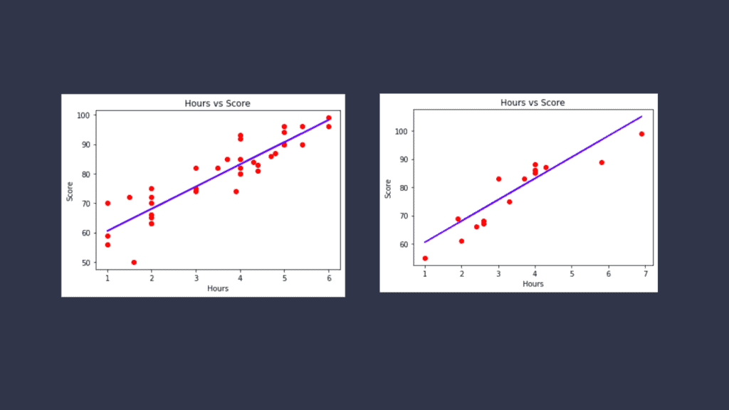
The above code shows the implementation of the Linear regression from importing the dataset, splitting it, and training the model, to visualize the results.

Evaluating the Linear Regression model

We already know that Linear Regression tries to fit a line that produces the smallest difference between predicted and actual values. We get the best-fit line from the training dataset. Different performance evaluation methods are used to know how close the predicted line is to the actual values. These methods help us calculate the linear regression model’s accuracy, precision, and f-score on the specific dataset.

A Machine Learning model cannot be 100% accurate; otherwise, it is biased. It is necessary to acquire accuracy in training data, but it is equally critical to obtain a genuine and approximate output on unknown data; otherwise, the model is useless. So, to construct and deploy a generalized model, we must evaluate it using various metrics to optimize, fine-tune it, and acquire a better outcome. We’ll discuss it later when we the concept of overfitting and underfitting.

Evaluation metrics measure how well a model performs and approximates the relationship. It quantifies the performance of a predictive model. This typically involves training a model on a dataset, then using the model to generate predictions on a holdout dataset that was not used during training, and comparing the predictions to the expected values in the holdout dataset. We will use MAE, MSE, RMSE, RMSLE, and R Squared measures to evaluate the performance of our model.

Mean Absolute Error (MAE)

The Mean Absolute Error (MAE) is the simplest regression error metric. It represents the average absolute difference between the actual and predicted values in the dataset. And measures the average of the residuals in the dataset.

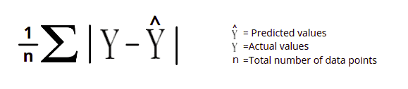
Let’s take sample data and calculate the mean absolute error. First, we will calculate the error (the difference between actual and predicted value), find the sum of absolute values of the errors, and divide by the total number of datasets.

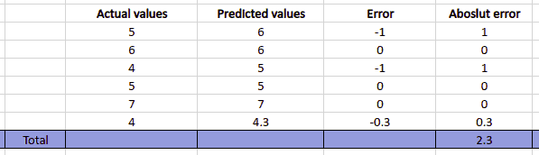
So the Mean Absolute Error in the above case will be 2.3/6 = 0.3833.

Now, let’s implement the MAE in Python for the above-given data:

# actual values
actual_values = [5,6,4,5,7,4]
# predicted avlues
predicted_values = [6,6,5,5,7,4.3]
# Importing mean_absolute_error from sklearn module
from sklearn.metrics import mean_squared_error, mean_absolute_error
# printing the mean absolute error
print(mean_absolute_error(actual_values, predicted_values))

Output:

Notice that we get the same result as we have found above. Let us now apply the same method and find the mean absolute error of our trained model.

# Importing mean_absolute_error from sklearn module
from sklearn.metrics import mean_squared_error, mean_absolute_error
# printing the mean absolute error
print(mean_absolute_error(y_test, y_pred))

Output:

y_test contains the actual values and y_pred contains the predicted values.

The advantage of using Mean Absolute Error is that all errors will be weighted on the same linear scale because we take the absolute value. That means we won’t place too much weight on our outliers, and our loss function provides a generic and consistent assessment of how well our model is doing. However, the MAE won’t be as effective if we care about our model’s outlier predictions. 

Mean Square Error (MSE)

The Mean Square Error (MSE) is similar to the Mean Absolute Error (MAE), but instead of taking the absolute value, it squares the difference before adding them together. The MSE will always be larger than the MAE because we squared the difference.

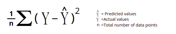
Using the above formula, let’s take sample data first and calculate the mean square error. First, we will calculate the error (the difference between the actual value and predicted value), find the sum of the square of the error, and divide the sum by the total number of datasets.

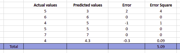
The Mean Square Error will be 5.09/6 = 0.84833.

Now, let’s implement the same method in Python:

# actual values
actual_values = [5,6,4,5,7,4]
# predicted avlues
predicted_values = [3,6,5,5,7,4.3]
# Importing mean_absolute_error from sklearn module
from sklearn.metrics import mean_squared_error, mean_absolute_error
# printing the mean squared error
print(mean_squared_error(actual_values, predicted_values))

Output:

Notice that we get the same result.

Let’s now apply the same method to our trained model and find out the mean square error of our model.

# Importing mean_absolute_error from sklearn module
from sklearn.metrics import mean_squared_error, mean_absolute_error
# printing the mean squared error
print(mean_squared_error(y_test, y_pred))

Output:

So the y_test and y_pred where the actual and predicted values are stored.

The MSE is useful for ensuring that our trained model does not contain any outlier predictions with significant errors, as the squaring element of the function gives these errors more weight. However, if our model makes a bad prediction, the squaring part of the function magnifies the error.

Root-Mean-Squared Error (RMSE)

It is similar to MSE, but RMSE is the square root of the average squared difference between the predicted and actual value. The only problem with MSE is that the loss order is higher than the data order. As a result, we can’t simply correlate data to the error. While in RMSE, we are not changing the loss function, and the solution is still the same. All we are doing is reducing the order of the loss function by taking root.

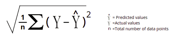
Now let us take sample data and calculate the root mean square error. We will follow the same procedure as the RME and then take the root of the final result.

The MRE value equals 0.8483 and is obtained by dividing the total error square by the total data points. To find the RMSE, we need to take the root of the MRE, and in the above case, the result will be 0.921.

Now, let us implement the same thing using the Python programming language.

# importing the square root method
from math import sqrt
# actual values
actual_values = [5,6,4,5,7,4]
# predicted avlues
predicted_values = [3,6,5,5,7,4.3]
# Importing mean_absolute_error from sklearn module
from sklearn.metrics import mean_squared_error
# printing the root mean absolute error
print(sqrt(mean_squared_error(actual_values, predicted_values)))

Output:

Notice that we get the same result.

Let us now determine the RMSE value of our trained model using the same procedure.

# importing square root method
from math import sqrt
# Importing mean_absolute_error from sklearn module
from sklearn.metrics import mean_squared_error, mean_absolute_error
# printing the mean squared error
print(sqrt(mean_squared_error(y_test, y_pred)))

Output:

y_test and y_pred are the actual output values and model-predicted output values, respectively.

R-Squared Error

The R-Squared Error method is also known as the coefficient of determination. This metric indicates how well a model fits a given dataset. Or in simple words, it indicates how close the regression line is to the actual data values. The R-Squared value lies between 0 and 1, where 0 indicates that this model doesn’t fit the given data and 1 means that the model perfectly fits the dataset provided.

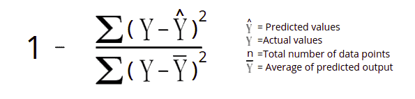
Let us now take a sample dataset and find out the R-squared Error. We will first calculate the sum of squared errors. Then will find the sum of the differences between the actual values and the predicted average value. Finally, we will subtract the divided value of these from 1.

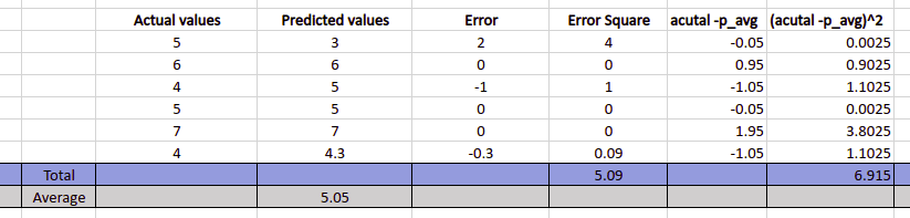
To calculate the R-Square error, we have to divide the sum of the error square by the sum of (actual-p_avg)^2 and subtract the result from 1. Which is equal to 1 - (5.09/6.915) = 0.263.

Now, let’s calculate the R-square error using Python.

# actual values
actual_values = [5,6,4,5,7,4]
# predicted avlues
predicted_values = [3,6,5,5,7,4.3]
# importing r square error
from sklearn.metrics import r2_score 
# applying r square error
R_square = r2_score(actual_values, predicted_values) 
print(R_square)

Output:

Now let us apply the same method to our trained model and find out the R-Squared Error of our model.

from sklearn.metrics import r2_score 
# applying r square error
R_square = r2_score(y_test, y_pred) 
print(R_square)

Output:

The y_test contains the actual values and the y_pred contains the predicted values.

Advantages and Disadvantages of Linear regression

Regression models are target prediction values based on independent variables. It is mostly used for finding out the relationship between variables and forecasting. Based on the performance and result, linear regression algorithms have pros and cons.

First, let’s discuss the pros of Linear regression:

• The Linear regression model uses the simplest equation to find the relationship between the multiple predictor variables and the predicted variables. The mathematical equations of Linear regression are also fairly easy to understand and interpret.
• Linear regression has significantly lower time complexity than some of the other Machine Learning algorithms. For example, modeling speed is fast in Linear regression since it does not require costly calculations and makes predictions quickly even when the amount of data is huge.
• Although Linear Regression is susceptible to over-fitting, it can be avoided using some dimensionality reduction techniques, regularization techniques, and cross-validation.

On the other hand, some of the cons of the Linear regression algorithm are as follows:

• Linear regression fails to fit complicated datasets because it assumes a linear relationship between the input and output variables. The relationship between the dataset’s variables isn’t linear in most real-world scenarios. Therefore, a straight line doesn’t appropriately fit the data.
• Outliers of a data set are anomalies or extreme values that deviate from the other data points of the distribution. Outliers can have a significant impact on the performance of linear regression. Hence they must be dealt with properly before Linear regression is used in the dataset.
• Linear Regression should not be used if the number of observations is less than the number of features. Otherwise, it may result in overfitting because it starts considering noise when developing the model.

Additional Learning Materials

From our point of view, these are the best hands-on online courses related to Machine Learning and Deep Learning available on the market right now:

Summary

Linear regression is one of the easiest and most popular Machine Learning algorithms. It makes predictions based on continuous variables. It uses a simple mathematical formula to train the model based on the training data. This article covered the implementation of the Linear Regression algorithm using Python language, AWS SageMaker Studio, and Jupyter Notebook.

We strongly recommend you check out the Complete Linear Regression Analysis in Python Udemy course for more in-depth information.