Random Forest Python Implementation Example

Random Forest Algorithm is an important algorithm because it helps reduce overfitting in models, improves predictive accuracy, and can be used for regression and classification problems. It also provides variable importance measures that indicate the most significant variables in a dataset and can be used for feature selection. Additionally, Random Forest Algorithm is easy to implement and has a low implementation cost.

This Random Forest Python tutorial overviews the Random Forest algorithm and demonstrates its Python implementation examples for binary and multiclass classification problems. Let’s get started!

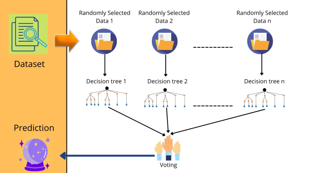
The Random Forests Algorithm is a Supervised learning algorithm. It can be utilized for classification and regression problems and is the most flexible and easy algorithm – the forest consists of trees. Random forests generate decision trees from randomly chosen samples, then obtain predictions from each tree and select the best option based on majority votes. 

Overview of Random Forest Algorithm

The concept of the Random Forest Algorithm is based on ensemble learning. Ensemble learning is a general meta-approach in Machine Learning that seeks better predictive performance by combining the predictions from multiple models. In simple words, It involves fitting many different model types on the same data and using another model to learn the best way to combine the predictions. So, Random Forest Algorithm combines predictions from decision trees and selects the best prediction among those trees.

We can define Random Forest as “a classifier that contains some decision trees on various subsets of the given dataset and takes the average to improve the predictive accuracy of that dataset.” Instead of relying on one decision tree, the algorithm takes the prediction from each tree, based on the majority votes of predictions, and forecasts the final output.

The following are the benefits of using the Random Forest Algorithm:

• It takes less training time as compared to other algorithms
• It predicts output with high accuracy, even for the large dataset
• It makes accurate predictions and runs efficiently
• It can also maintain accuracy when a large proportion of data is missing
• It does not suffer from the overfitting problem because it takes the average of all the predictions, which cancels out the biases
• The algorithm can be used in both classification and regression problems
• We can get the relative feature importance using Random Forest Algorithm, which helps in selecting the most contributing features for the classifier

How does Random Forest Algorithm Work?

The Random Forest Algrothim builds different decision trees on a randomly selected dataset and takes one of the decision trees based on the majority voting. For more information on the implementation of decision trees, check out our article “Implementing Decision Tree Using Python.” The Random Forest Algorithm consists of the following steps:

1. Random data selection – the algorithm selects random samples from the provided dataset
2. Building decision trees – the algorithm creates a decision tree for each selected sample
3. Get a prediction result from each of created decision tree
4. Perform voting for every predicted result
5. Select the most voted prediction result as the final prediction

Random Forest Python Example – Binary classification

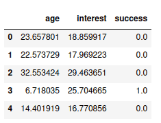
Let’s implement the Random Forest Algorithm for the binary classification problem. Binary classification is a classification in which there are only two output categories. In this section, we will use a sample binary dataset that contains the age and interest of a person as independent/input variables and the success as an output class.

First, let us import the data and view some of the data by using the pandas module.

# importing the pandas module
import pandas as pd
# importing the data set
data = pd.read_csv('RandomForest.csv')
# printing the fist few data set
data.head()

Output:

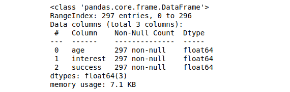
We can get more information about the dataset (type, memory, null values, etc.) by using the info() method:

# getting the information about dataset
data.info()

Output:

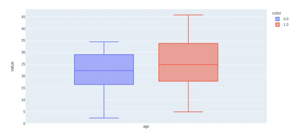
Visualizing the dataset

We can visualize the dataset in many ways to get an idea about the data set and the relation between the input and output variables. First, we visualize the input variable ‘age’ and the output class using a box plot.

# Importing the plotly module
import plotly.express as pt
# ploting box graph ( age and success)
pt.box(data["age"], color=data["success"])

Output:

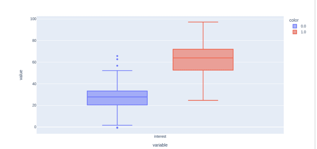
Let us build the same box graph for the input variable “interest” and output classes.

# Importing the plotly module
import plotly.express as pt
# ploting box graph ( age and success)
pt.box(data["interest"], color=data["success"])

Output:

Now, let’s visualize the data using a pie chart to see if our data is unbalanced or not.

# importing numpy
import numpy as np
import matplotlib.pyplot as plt
# creating variables
class_one = 0
class_two = 0
# for loop to itreate through the output class
for i in data['success']:
    if i ==0:
        class_one+=1
    else:
        class_two+=1
# creating numpy arry
values = np.array([class_one, class_two])
label = ["No Success", "success"]
# ploting the graph
plt.pie(values, labels = label)
plt.show()
# printing the results
print("No-Success : ", class_one)
print("Success  :", class_two)

Output:

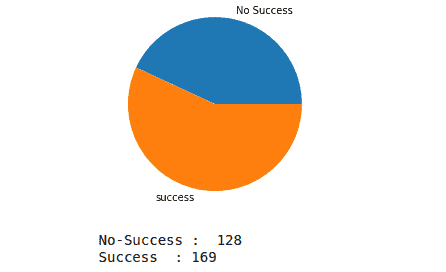
As you can see, the dataset is slightly unbalanced, but it’s ok for our example.

Training and Testing of the model

Before feeding the data to our model to train, we must extract the input/independent variables and output/dependent classes in separate variables.

# dividing the dataset into inputs and outputs
y = data[["success"]]
X = data.drop(columns=["success"])

The next step is splitting the given dataset into training and testing datasets so we can later use the data to evaluate the model’s performance.

# training and testing data
from sklearn.model_selection import train_test_split
# assign test data size 20%
X_train, X_test, y_train, y_test =train_test_split(X,y,test_size= 0.2, random_state=0)

Scaling the dataset before feeding it to the model is critical in Machine Learning as it reduces the effect of outliers on the model’s predictions.

# Importing standardScaler
from sklearn.preprocessing import StandardScaler
# scalling the input data
sc_X = StandardScaler() 
X_train = sc_X.fit_transform(X_train)
X_test = sc_X.fit_transform(X_test)

After scaling, we can feed the training data to the Random Forest Python sklearn classifier to train the model.

# import Random Forest classifier
from sklearn.ensemble import RandomForestClassifier
# instantiate the classifier 
classifier = RandomForestClassifier()
# fit the model
classifier.fit(X_train, y_train)

Now our model is trained, we can provide any input values to predict the output ( success or not-success).

# predicting the outcome
y_output = classifier.predict([[19, 19.43]])
# printing the output
print(y_output)

Output:

The output shows the person who will succeed based on provided input values. But we don’t know how much the prediction is accurate. To get the model’s accuracy, we need a testing dataset:

# testing the model
y_pred = classifier.predict(X_test)
# importing accuracy score
from sklearn.metrics import accuracy_score
# printing the accuracy of the model
print(accuracy_score(y_test, y_pred))

Output:

The output shows that our model is 90% accurate.

Visualizing the training set

Here we will visualize the training set result. We will plot a graph for the Random Forest classifier to visualize the training set result. The classifier will predict Yes or No for the users who have either Success or Not success.

# importing modules
import numpy as np
from matplotlib.colors import ListedColormap  
# converting the output to 1d array
result = np.array(y_train).flatten()
# seting x_train and y_train
x_set, y_set = X_train, result  
x1, x2 = np.meshgrid(np.arange(start = x_set[:, 0].min() - 1, stop = x_set[:, 0].max() + 1, step  =0.01),  
np.arange(start = x_set[:, 1].min() - 1, stop = x_set[:, 1].max() + 1, step = 0.01))  
# Ploting 
plt.contourf(x1, x2, classifier.predict(np.array([x1.ravel(), x2.ravel()]).T).reshape(x1.shape),  
alpha = 0.75, cmap = ListedColormap(('blue','yellow' )))  
plt.xlim(x1.min(), x1.max())  
plt.ylim(x2.min(), x2.max())  
# for loop to iterate the data
for i, j in enumerate(np.unique(y_set)):  
    plt.scatter(x_set[y_set == j, 0], x_set[y_set == j, 1],  
        c = ListedColormap(('black', 'red'))(i), label = j) 
    
# labeling the graph
plt.title('Random forest training set')  
plt.xlabel('Age')  
plt.ylabel('Interest')  
plt.legend()  
plt.show()

Output:

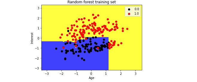
The above image is the visualization result for the Random Forest classifier working with the training set result. Each data point corresponds to a person’s data; the blue and yellow regions are the prediction regions. The yellow area shows the successful people, and the blue part shows people who are not.

Visualizing the testing set

Now let’s visualize the testing dataset of the model. The code will be pretty similar. All we need to do is replace X_train and y_train with X_test and y_test:

# converting the output to 1d array
result = np.array(y_test).flatten()
# seting x_train and y_train
x_set, y_set = X_test, result  
x1, x2 = np.meshgrid(np.arange(start = x_set[:, 0].min() - 1, stop = x_set[:, 0].max() + 1, step  =0.01),  
np.arange(start = x_set[:, 1].min() - 1, stop = x_set[:, 1].max() + 1, step = 0.01))  
# Ploting 
plt.contourf(x1, x2, classifier.predict(np.array([x1.ravel(), x2.ravel()]).T).reshape(x1.shape),  
alpha = 0.75, cmap = ListedColormap(('blue','yellow' )))  
plt.xlim(x1.min(), x1.max())  
plt.ylim(x2.min(), x2.max())  
# for loop to iterate the data
for i, j in enumerate(np.unique(y_set)):  
    plt.scatter(x_set[y_set == j, 0], x_set[y_set == j, 1],  
        c = ListedColormap(('black', 'red'))(i), label = j) 
    
# labeling the graph
plt.title('Random forest training set')  
plt.xlabel('Age')  
plt.ylabel('Interest')  
plt.legend()  
plt.show()

Output:

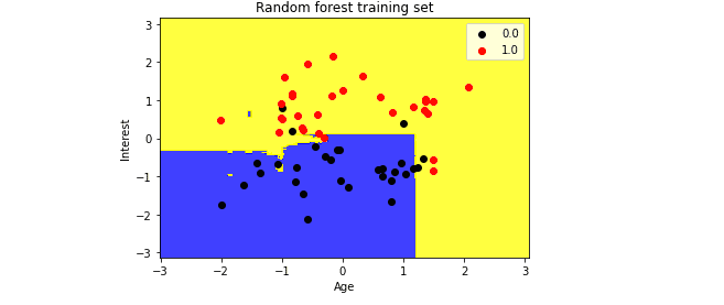
So, any input data point in the blue region is considered “no success,” and the yellow area will represent “success.”

Evaluation of Random Forest for binary classification

Let us now evaluate the performance of our model. We will use a confusion matrix to evaluate the model. A confusion matrix summarizes correct and incorrect predictions, which helps us calculate accuracy, precision, recall, and f1-score. It contains TP, TN, FP, and FP values.

# importing the required modules
import matplotlib.pyplot as plt
from sklearn.metrics import confusion_matrix, ConfusionMatrixDisplay
# Plot the confusion matrix in graph
cm = confusion_matrix(y_test,y_pred, labels=classifier.classes_)
# ploting with labels
disp = ConfusionMatrixDisplay(confusion_matrix=cm, display_labels=classifier.classes_)
disp.plot()
# showing the matrix
plt.show()

Output:

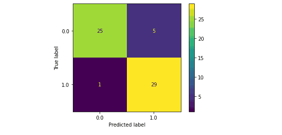
The confusion matrix shows that the model correctly predicted 25 out of 30 “no success” classes and 29 out of 30 “success” classes.

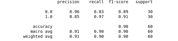
Let us not check the classification report of the model.

# Importing classification report
from sklearn.metrics import classification_report
# printing the report
print(classification_report(y_test, y_pred))

Output:

Random Forest Python Example – Multiclass classification

Multiclass classification is a classification with more than two output classes. In this section, we will use a multi-classification dataset. Let’s load the dataset and print out the first few rows using the pandas module.

# importing the dataset
df = pd.read_csv('RamdonForestMulticlass.csv')
# print 5 rows
print(df.head(5))

Output:

The output shows that our dataset contains 22 columns with 21 independent variables (number of columns).

Exploring and visualizing dataset

First, let us check if our data set has any missing values because we came across data with missing values in most real-life cases.

# checking for missing values
df.isna().sum()

Output:

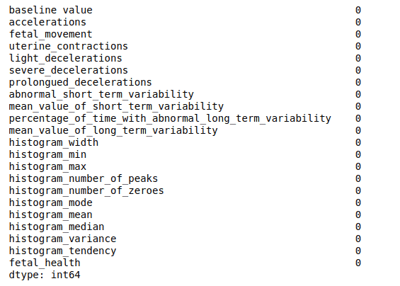
So there are no missing values in our dataset.

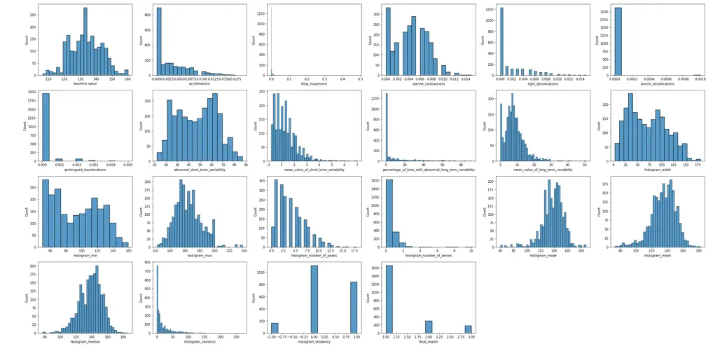
Let’s visualize each of the columns (features).

# importing required modules
import seaborn as sns
# figure sizes
plt.figure(figsize=(30, 15))
# for loop to interate through columns
for i, column in enumerate(df.columns):
    plt.subplot(4, 6, i + 1)
    sns.histplot(data=df[column])
# showing the graphs
plt.tight_layout()
plt.show()

Output:

If there are any, let’s visualize the dataset outliers using the box plot method. An outlier is a data point that differs significantly from other observations.

# size of the graph
plt.figure(figsize=(30,10))
# ploting the box plot
sns.boxplot(data = df,palette = "Set1")
plt.xticks(rotation=90)
# showing the graph
plt.show()

Output:

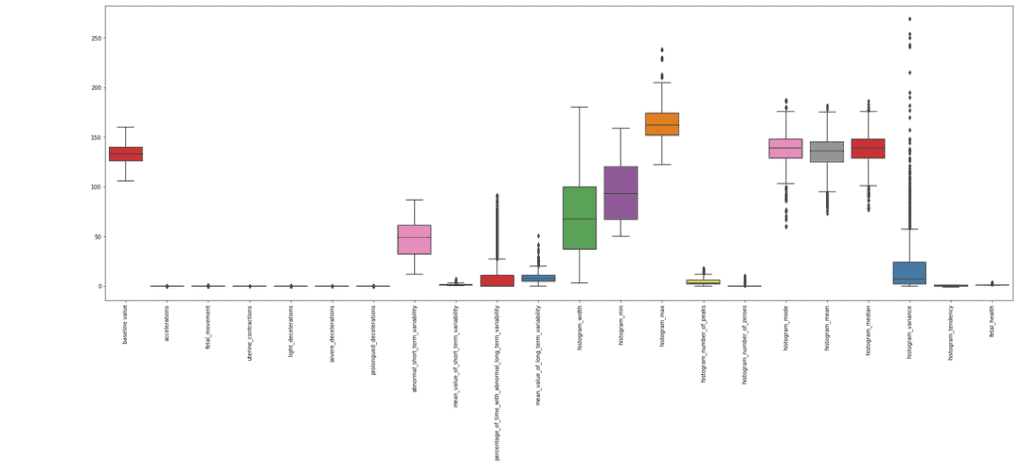
The graph shows that there are a lot of outliers that can affect the predictions. We can write our function to remove these outliers.

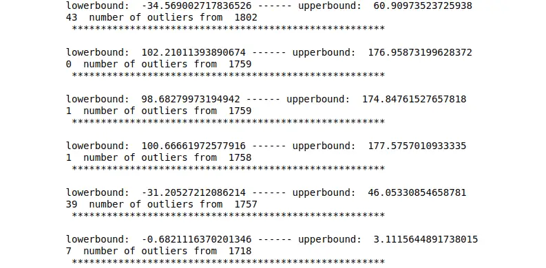
# Function to set upper and lower bound to 3rd standard deviation and remove outliers
def removeOutlier(attribute, df):
    # lower and upper bound
    lowerbound = attribute.mean() - 3 * attribute.std()
    upperbound = attribute.mean() + 3 * attribute.std()
    print('lowerbound: ',lowerbound,'------ upperbound: ', upperbound )
    
    # checkting for outliers
    df1 = df[(attribute > lowerbound) & (attribute < upperbound)]
    # printing
    print((df.shape[0] - df1.shape[0]), ' number of outliers from ', df.shape[0] )
    print(' ******************************************************\n')
    
    # creating copy
    df = df1.copy()
    # return the dataframe
    return df
# calling the function
df = removeOutlier(df.histogram_variance, df)
df = removeOutlier(df.histogram_median, df)
df = removeOutlier(df.histogram_mean, df)
df = removeOutlier(df.histogram_mode, df)
df = removeOutlier(df.percentage_of_time_with_abnormal_long_term_variability, df)
df = removeOutlier(df.mean_value_of_short_term_variability, df)

Output:

Now, let’s plot the box plot and see the difference.

# size of the graph
plt.figure(figsize=(30,10))
# the box plot
sns.boxplot(data = df,palette = "Set1")
plt.xticks(rotation=90)
# showing graph
plt.show()

Output:

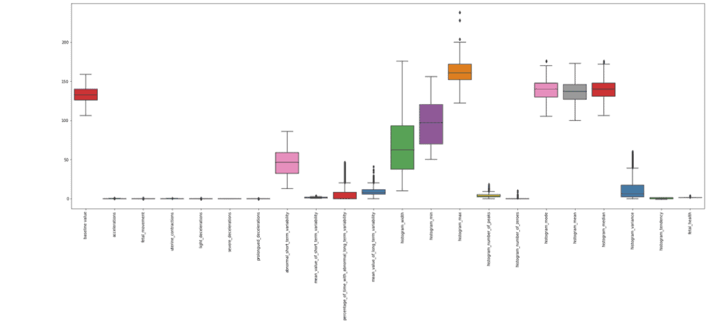
Notice that there are fewer outliers this time compared to the previous one.

Training and Testing the model

Before feeding the data to the model, we must separate the inputs and outputs and store them in different variables.

# contains all the columns except the last one
x = df.drop('fetal_health', axis = 1)
# contain only last column
y = df['fetal_health'] 

The next step is to split the dataset into training and testing parts to evaluate the model’s performance.

# importing the module
from sklearn.model_selection import train_test_split
# spliting the dataset
x_train, x_test, y_train, y_test = train_test_split(x,y,test_size = 0.25, random_state = 0)

Note: We assigned 75% of the data to the training and only 25% to the testing.

Let us now scale our data so that the outliers do not have too much effect.

# importing the module
from sklearn.preprocessing import StandardScaler
# initializing the standard scalling method
scaler = StandardScaler()
# scalling the input values
x_train = scaler.fit_transform(x_train)
x_test = scaler.transform(x_test)

After scaling, the data is ready for training the model. Let’s import the random forest classifier and train the model.

# import Random Forest classifier
from sklearn.ensemble import RandomForestClassifier
# instantiate the classifier 
classifier = RandomForestClassifier()
# fit the model
classifier.fit(x_train, y_train)

Let’s test our model by providing the testing dataset.

# testing the model
y_pred = classifier.predict(x_test)
# importing accuracy score
from sklearn.metrics import accuracy_score
# printing the accuracy of the model
print(accuracy_score(y_test, y_pred))

Output:

The accuracy of the model is 92% which is pretty high.

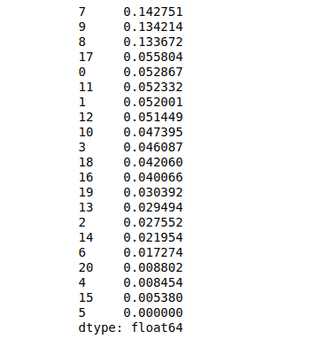
Sorting features by importance using sklearn

Let’s find which features from the dataset are more critical than the others:

# importing pandas
import pandas as pd
# classifing the features according to their importance
feature_imp = pd.Series(classifier.feature_importances_,index=[i for i in range(21)]).sort_values(ascending=False)
# printing
print(feature_imp)

Output:

We can also visualize these important features to understand them better. For visualization, we will use a combination of matplotlib and seaborn. The seaborn library is built on top of matplotlib, and it offers several customized themes and provides additional plot types.

# importing the modules
import matplotlib.pyplot as plt
import seaborn as sns
# graph size
plt.figure(figsize=(30,10))
# Creating a bar plot
sns.barplot(x=feature_imp, y=feature_imp.index)
# Add labels to your graph
plt.xlabel('Feature Importance Score')
plt.ylabel('Features')
plt.title("Visualizing Important Features")
plt.show()

Output:

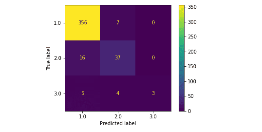
Model evaluation using a confusion matrix

Let’s evaluate the model you trained using a multiclass classification dataset. We will use seaborn module to visualize the confusion matrix.

# importing the required modules
import matplotlib.pyplot as plt
from sklearn.metrics import confusion_matrix, ConfusionMatrixDisplay
# Plot the confusion matrix in graph
cm = confusion_matrix(y_test,y_pred, labels=classifier.classes_)
# ploting with labels
disp = ConfusionMatrixDisplay(confusion_matrix=cm, display_labels=classifier.classes_)
disp.plot()
# showing the matrix
plt.show()

Output:

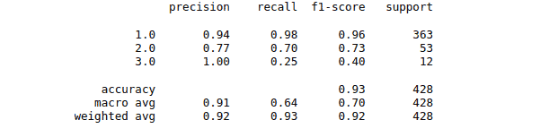
Let us print the classification report of our model, which will help us evaluate its performance.

# Importing classification report
from sklearn.metrics import classification_report
# printing the report
print(classification_report(y_test, y_pred))

Output:

Random Forest Aglroithm using sklearn and AWS SageMaker Studio

Let’s implement the Random Forest Algorithm using SageMaker Studio and Python version 3.7.10. Here’s a complete code for the Random Forest Algorithm:

# importing the pandas module
import pandas as pd
# importing the data set
data = pd.read_csv('RandomForest.csv')
# dividint the dataset into inputs and outputs
y = data[["success"]]
X = data.drop(columns=["success"])
#Training and testing data
from sklearn.model_selection import train_test_split
# assign test data size 20%
X_train, X_test, y_train, y_test =train_test_split(X,y,test_size= 0.3, random_state=1)
# Importing standardScaler
from sklearn.preprocessing import StandardScaler
# scalling the input data
sc_X = StandardScaler() 
X_train = sc_X.fit_transform(X_train)
X_test = sc_X.fit_transform(X_test)
# import Random Forest classifier
from sklearn.ensemble import RandomForestClassifier
# instantiate the classifier 
classifier = RandomForestClassifier()
# fit the model
classifier.fit(X_train, y_train)
# testing the model
y_pred = classifier.predict(X_test)
# importing accuracy score
from sklearn.metrics import accuracy_score
# printing the accuracy of the model
print(accuracy_score(y_test, y_pred))

Output:

FAQ

Summary

Random Forest is a commonly-used Machine Learning algorithm that combines the output of multiple decision trees to reach a single result. This article covered the Random Forest Algorithm, its Python implementation, and the evaluation of the model using a confusion matrix. We also used the services of AWS SageMaker for the implementation and visualization parts.