Gaussian Process For Classification and Regression

The Gaussian process is a robust Supervised Machine Learning algorithm used to solve regression and classification problems. It assumes that the underlying data is normally distributed and normally jointly distributed. This article will describe how to use the Gaussian process regressor and classifier, apply them to datasets and review the results. We will be using AWS SageMaker Studio and Jupyter notebooks for implementation and visualization purposes.

We assume that you are already familiar with the normal distribution and probabilities. The Gaussian process uses them to make predictions, and we will rely on these concepts in our article. We also recommend you review the Naive Bayes algorithm before learning the Gaussian process because the Gaussian process solves classification problems using Naive Bayes.

Explanation of Gaussian process classifier

A classifier is a model used to make predictions trained on a classification dataset. So, here we will explain how the Gaussian process classifies the categorical values.

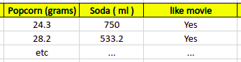
Let’s take a sample classification dataset and then review how the Gaussian process classifier is trained. We can use a dataset containing the information on whether people liked the movie or not. Let’s assume that the amount of eaten popcorn and amount of drunken soda are features defining the output variable (if the person will like the movie).

The entire dataset might be split equally to the one that has only positive outcomes:

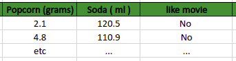
And the one that contains only negative outcomes:

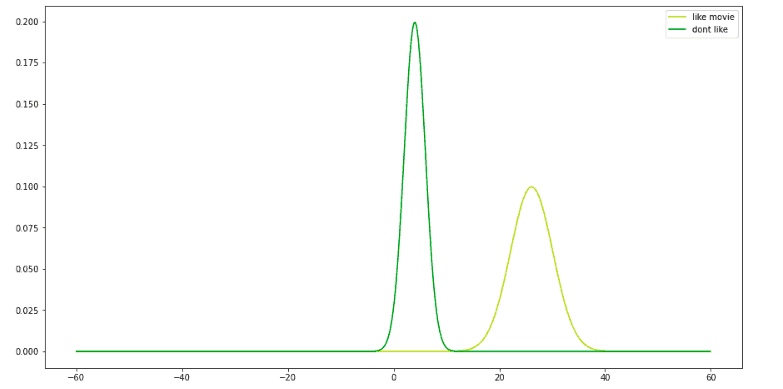
For each dataset, the algorithm calculates the mean and standard deviation of each independent variable to find out its normal distribution. For example, the mean and standard deviation of values in the popcorn column for the people who like the movie is 26.25 and 2.76. The mean and standard deviation values of the popcorn column for the people who didn’t like the movie are 3.45 and 1.91.

The normal distribution of popcorn values for both categories looks like this:

Similarly, the algorithm calculates the mean and standard deviation for the values of the soda column. Let’s say we have the following normal distribution of the soda column values for each output class:

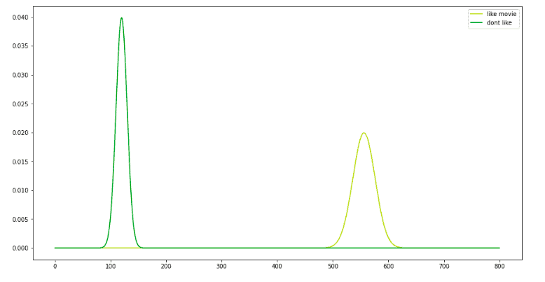
Normal distributions above help us predict whether a person will like the movie or not.

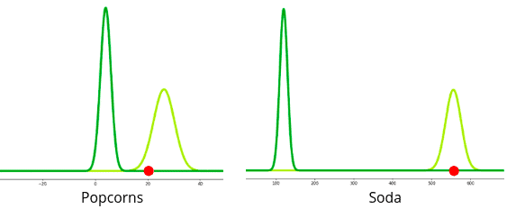
For example, let’s predict whether the person will like the movie or not if a person will eat 20 grams of popcorn and drink 550 ml of soda.

Let’s plot the input data on top of the above distributions:

Now the Gaussian process has to perform some probabilities calculations. It starts its prediction from the initial guess. The initial guess will be the overall probability of liking the not liking the movie based on the output of the training dataset.

P ( like movie ) = 0.5

P ( not like ) = 0.5

The initial guess in our case is 0.5 because we are assuming that the dataset contains an equal number of people who liked the movie and who didn’t like the movie. These initial guesses are called prior probabilities.

Now we can calculate the total score for both classes. The following equation is used to calculate the total score for the person to like the movie:

Note: The L represents the likelihood function for our input data points.

So, the total score will be:

Like movie = 0.5 * 0.02 * 0.006

Because we have very small numbers, let’s use the log function:

like movie = log ( 0.5 * 0.02 * 0.006 )

We assume that you already know how the log function works:

like movie = log 0.5 + log 0.02 + log 0.006

like movie = (-3) + ( -1.69 ) + (- 2.22 ) = -6.91

Similarly, the algorithm will calculate the total score for not liking the movie using the following formula:

So, the total score will be:

Don’t like the movie = 0.5 * very small number * very small number

Let us assume that these very small numbers are 0.00001.

Don’t like the movie = log(0.5) + log( 0.00001 ) + log( 0.00001 )

Don’t like the movie = (-3) + ( -5 ) + ( -5 ) = -13

The score of liking the movie based on the input data (20 grams of popcorn and 550 ml of soda) is higher than the total score for not liking the movie. As a result, the algorithm will classify the person who consumes 20 grams of popcorn and 550 ml of soda as the one who will like the movie.

Explanation of Gaussian process regressor

A regression problem is a dataset containing continuous value output rather than categorical. In the case of a regression problem, the algorithm tries to find a function that best fits the training dataset.

In this section of the article, we will review how the Gaussian process regressor finds the best-fitted line for the regression dataset. We will not go deep into the mathematical calculations. Instead, we will use different graphs to understand the Gaussian process regressor actions.

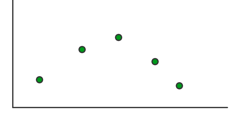
Let’s assume that we have the following training dataset.

Any regression model aims to find the best-fitted function for the given data. In the case of the Gaussian process, it will find all the possible functions that can fit the above dataset. Let’s imagine it comes up with the following functions:

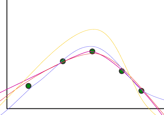
The next step will find the mean of these functions, which will be the best-fitted function for the given training dataset.

Let’s say the following is the mean of the above functions.

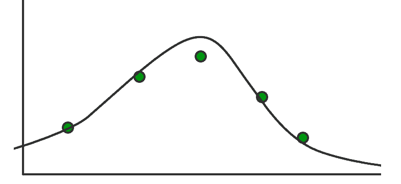
This will be the best-fitted line, and all the predictions will be outcomes of this function.

Data classification using the Gaussian process

A classification dataset is a dataset that contains categorical output as target variables. We will use the wine dataset from the sklearn module as a sample dataset to train the Gaussian process classifier. The dataset contains information about three different wines.

Before going to the implementation part, make sure that you have installed the following modules on your system as we will be using them.

• sklearn
• numpy
• pandas
• matplotlib

You can install the required modules by running the following commands in the cell of the Jupyter notebook.

%pip install sklearn
%pip install pandas
%pip instal numpy
%pip install matplotlib

Once the installation is complete, we can go with the implementation part.

Importing and exploring the dataset

Let’s load the dataset from the sklearn module.

# importing the wine dataset
from sklearn.datasets import load_wine
import pandas as pd
# loading the dataset
wine=load_wine()
#converting the data to dataframe
data=pd.DataFrame(data=np.c_[wine['data'],wine['target']],columns=wine['feature_names']+['target'])
# checking the heading
data.shape

Output:

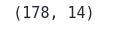
This shows that the dataset contains a total of 178 observations and 14 columns.

Let’s now check if we have any null values. We can use the pandas’ isnull() method to find it out.

# finding the null values
data.isnull().sum()

Output:

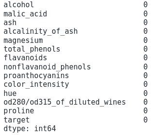
The output shows that there are no null values in the dataset.

We can use the bar plot to check if the output values are balanced or not.

#Convert the target variable to categorical.
data.target=data.target.astype('int64').astype('category')
#finding the frequency 
freq=data['target'].value_counts()
#plotting the bar graph
freq.plot(kind='bar')

Output:

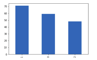
Although the data is not perfectly balanced, still it is balanced enough to be used to train the model.

Splitting the dataset

Let’s extract input variables (features) and output variables:

# input and output
Input, output = load_wine(return_X_y=True)

The next step is to split the dataset into training and testing parts:

# importing the module
from sklearn.model_selection import train_test_split
# splitting the dataset
X_train, X_test, y_train, y_test = train_test_split(Input, output, test_size=0.20)

We’ll use 20% of the data for testing and the remaining 80% for training.

Training and testing the Gaussian process classifier

Let’s train the model using the training dataset:

# importing the required module
from sklearn.gaussian_process import GaussianProcessClassifier
# initializing the classifier
model = GaussianProcessClassifier()
# training the model
model.fit(X_train, y_train)

Once the training is complete, we can predict the output by providing the testing dataset.

# predictions
prediction = model.predict(X_test)

We have stored the predictions in a variable.

Evaluating the Gaussian process classifier

We will use a confusion matrix to evaluate the classifier. It is a method of summarizing a classification algorithm’s performance. It is simply a summarized table of the number of correct and incorrect predictions. Calculating a confusion matrix can give us a better idea about the miss-classified classes. We can easily determine the model’s accuracy by examining the diagonal values by visualizing the confusion matrix.

The confusion matrix of the Gaussian process classifier is:

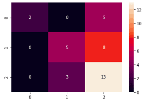
The confusion matrix shows that the model is not very good at predicting the third type of wine. Because most of the misclassification has occurred in the third type of wine.

Let’s now calculate the accuracy of the model as well.

# importing accuracy score
from sklearn.metrics import accuracy_score
# accuracy
accuracy_score(y_test,prediction)

Output:

This shows that only 55% of the data points from the testing data were classified correctly, which is very low.

Applying GridSearchCV

The accuracy of the model is very low, we can apply GridSearchCV helper class to find the optimum parameter for the kernel. The Gaussian process uses the kernel to define the covariance of a prior distribution over the target functions and uses the observed training data to define a likelihood function. As GridSearachCV takes time to find the optimum parameters when applied to many parameters, we will apply them to the kernel parameter only.

First, let’s create a function that will show how much time it takes for the GridSearchCV to find the best parameters:

# function to print the total time
def timer(start_time=None):
    # starting the time
    if not start_time:
        start_time = datetime.now()
        return start_time
    # ending the time
    elif start_time:
        thour, temp_sec = divmod((datetime.now() - start_time).total_seconds(), 3600)
        tmin, tsec = divmod(temp_sec, 60)
        # printing the total time
        print('\n Time taken: %i hours %i minutes and %s seconds.' % (thour, tmin, round(tsec, 2)))

Now we can import all the kernels available in the sklearn module and store them in a dictionary.

# importing the modules
from sklearn.gaussian_process.kernels import RBF, DotProduct, Matern, RationalQuadratic, WhiteKernel
# define grid
grid = dict()
grid['kernel'] = [1*RBF(), 1*DotProduct(), 1*Matern(),  1*RationalQuadratic(), 1*WhiteKernel()]

Let’s apply the GridSearchCV to find the best kernel for our dataset.

# importing required module
from sklearn.model_selection import GridSearchCV
from datetime import datetime
model = GaussianProcessClassifier()
# applying GridSearchCV
model=GridSearchCV(model, grid, scoring='accuracy')
# timing starts from this point for "start_time" variable
start_time = timer(None) 
# training the model
model.fit(X_train,y_train)
# timing ends here for "start_time" variable
timer(start_time) 
# printing the best estimator
print("\nThe best estimator returned by GridSearch CV is:",model.best_estimator_)

Output:

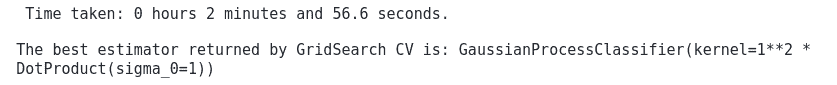
The GridSearchCV took 2 minutes and 56 seconds to find the best kernel for the dataset.

Using optimum kernel

Let’s train the model using the optimum kernel value that the GridSearchCV returned:

# define model
model_optimum = GaussianProcessClassifier(kernel=1**2 * DotProduct(sigma_0=1))
# training the model
model_optimum.fit(X_train,y_train)

Once the training is complete, we can use the testing data to predict the output values.

#  predictions
prediction_optimum = model.predict(X_test)

Let’s use the confusion matrix to see if our model improved:

# providing actual and predicted values
cm = confusion_matrix(y_test, prediction_optimum)
# If True, write the data value in each cell
sns.heatmap(cm,annot=True)
# saving confusion matrix in png form
plt.savefig('confusion_Matrix.png')

Output:

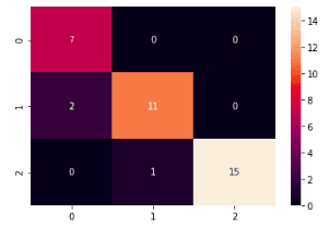
Notice that our model has performed exceptionally well on the third type of wine this time.

Let’s calculate the accuracy score too:

# accuracy
accuracy_score(y_test,prediction_optimum)

Output:

This time, our model’s accuracy is much higher.

Making predictions using the Gaussian process

A regression dataset contains data having continuous output values. In this section of the article, we will use a houses dataset and try to make house price predictions. The price of a house depends on the area, location, number of floors, and rooms. You can get access to the dataset using this link.

Importing and exploring the dataset

We will use the Pandas library to import the dataset and print out a few rows to get familiar with the dataset type:

# importing the module
import pandas as pd
# importing the dataset
dushanbe = pd.read_csv('Dushanbe_house.csv')
# heading
dushanbe.head()

Output:

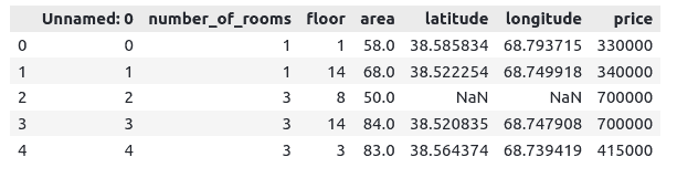
Notice that we have one column named ‘Unnamed: 0’, containing the index values. We don’t need this column, so that we will remove this from our dataset.

# dropping the column
dushanbe.drop('Unnamed: 0', axis=1, inplace=True)

Also, our dataset contains some null values. We will also remove them from the dataset.

# removing null values
dushanbe.dropna(inplace=True)
# checking null values
dushanbe.isnull().sum()

Output:

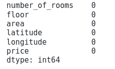
Notice that there are no null values anymore in the dataset.

We can use a box plot to check the distribution of the prices in the output category.

# importing the module
import seaborn as sns
# setting the theme stype
sns.set_theme(style="whitegrid")
# setting the size of plot
sns.set(rc = {'figure.figsize':(15,8)})
# plotting the boxplot
ax = sns.boxplot(x=dushanbe["price"])

Output:

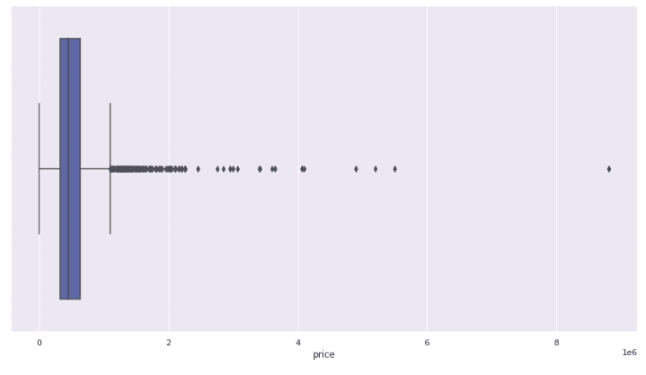
This shows that there are some outliers in the dataset. If you want to know how to handle outliers in a dataset, please check the article detection of anomaly objects using Python.

Splitting the dataset

We need to divide the dataset into input variables and output variables.

# splitting our dataset into independent and dependent variables
x_data = dushanbe.drop('price', axis=1)
y_data = dushanbe.price

The next step is to split the dataset into training and testing parts. We will assign 25% of the data for testing and 75% for the training.

# importing the module
from sklearn.model_selection import train_test_split
# splitting the dataset
X_train, X_test, y_train, y_test = train_test_split(x_data, y_data, test_size = 0.25, random_state = 0)

We can also check the size of the testing and training dataset by using the shape method.

# printing
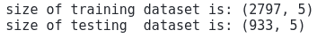
print("size of training dataset is:", X_train.shape)
print("size of testing  dataset is:", X_test.shape)

Output:

Training and testing Gaussian process classifier

Let’s train the model using the training dataset.

# importing the module
from sklearn.gaussian_process import GaussianProcessRegressor
# initializing the algorithm with default parameters
gp_regressor = GaussianProcessRegressor()
# training the model
gp_regressor.fit(X_train, y_train)

Once the training is complete, we can use the testing data to make predictions.

# predicting
gp_predictions = gp_regressor.predict(X_test)

As soon as we have predicted the values, we can visualize both the actual and predicted values on a plot to see how accurate the predicted values are:

# importing the module
import matplotlib.pyplot as plt
# fitting the size of the plot
plt.figure(figsize=(20, 8))
# plotting the graphs
plt.plot([i for i in range(len(y_test))],y_test, label="actual values", c='r')
plt.plot([i for i in range(len(y_test))],gp_predictions, label="Predicted values", c='g')
# showing the plotting
plt.legend()
plt.show()

Output:

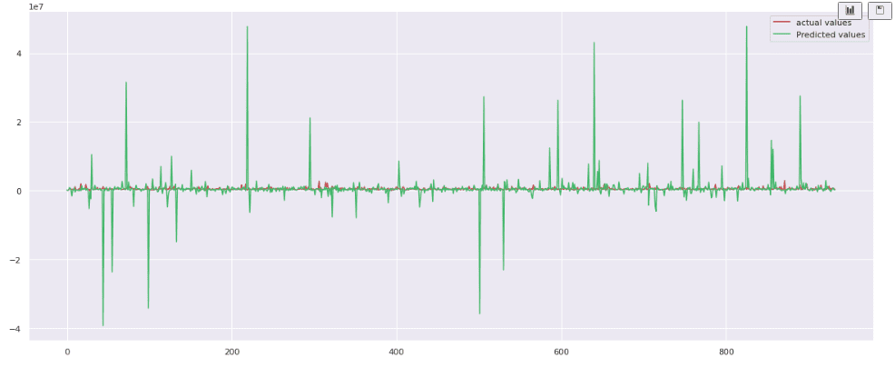
The plot shows that the model fails to follow the actual values. Let’s calculate the R-square score:

# Importing the required module
from sklearn.metrics import r2_score
# Evaluating the model
print('R score is :', r2_score(y_test, gp_predictions))

Output:

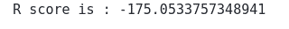
Usually, the R-square score is between 0 and 1. The closer the value is to the 1, the better the predictions are. But if the R-square value is a negative number, the model failed to follow the pattern.

Gaussian process regressor with custom kernel

We can change the kernel and train the model again to try to get better predictions.

# importing the modeul
from sklearn.gaussian_process.kernels import DotProduct, WhiteKernel
# setting the kernel
kernel = DotProduct() + WhiteKernel()

Let’s now the Gaussian process regressor using the above kernel.

# importing the module
from sklearn.gaussian_process import GaussianProcessRegressor
# trainining the model
gp = GaussianProcessRegressor(kernel=kernel)
# training the model
gp.fit(X_train, y_train)

We will use the testing data to make predictions.

# predicting
gp_p= gp.predict(X_test)

Let’s now plot the predictions and the actual values as we did previously.

# fitting the size of the plot
plt.figure(figsize=(20, 8))
# plotting the graphs
plt.plot([i for i in range(len(y_test))],y_test, label="actual values", c='r')
plt.plot([i for i in range(len(y_test))],gp_p, label="Predicted values", c='g')
# showing the plotting
plt.legend()
plt.show()

Output:

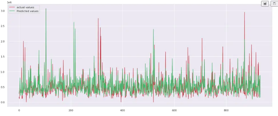
The plot shows that the predictions are much better this time. We can also calculate the R-square score to see how well the new model behaves.

# Evaluating the model
print('R score is :', r2_score(y_test, gp_p))

Output:

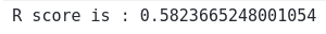
As we get a positive value which means this time, the predictions were much better than the previous one.

Summary

Gaussian Process is a Machine Learning technique used for regression and classification problems. Being a Bayesian method, Gaussian Process makes predictions with uncertainty. This article covered the Gaussian process in-depth and its strategy for solving classification and regression problems.