Using the ARIMA model and Python for Time Series forecasting
ARIMA is a statistical model that is used for time series analysis. The ARIMA model generalizes the ARMA model used for stationary time series. The ARIMA model can be used for non-stationary time series, but you must differentiate it first. This article will discuss the working and essential terms related to the ARIMA model. Also, we will implement the ARIMA model on a non-stationary time-series dataset.
Table of contents
You can also look at the Facebook Prophet, a time series predictive algorithm.
Understanding the terms used in the ARIMA model
ARIMA stands for AutoRegressive Integrated Moving Average. It is used to forecast future time series values based on past time series values. The ARIMA model can model stationary time series and non-stationary time series. It is a generalization of the ARMA model and the AR model. The ARMA model forecasts future time series values based on previous and past error term values. The ARIMA model can predict future values of a time series based on the last values of the time series, past values of the error terms, and past values of the differenced time series.
ARIMA models are generally denoted as ARIMA (p, d, q), where p is the order of the autoregressive model (AR), d is the degree of differencing, and q is the order of the moving-average model(MA). ARIMA model uses differencing to convert a non-stationary time series into a stationary one and then predict future values from historical data. The model uses “auto” correlations and moving averages over residual errors in the data to forecast future values.
Now, let us understand the terms commonly used with the ARIMA model.
What is the autoregressive (AR) model?
An autoregressive (AR) model predicts future behavior based on past behavior. It is used for forecasting when there is some correlation between values in a time series and values that precede and succeed.
Or we can also say that an autoregressive model is a model where Yt depends only on its lags. The Yt is a function of the ‘lags of Yt.’ A lag is a fixed amount of passing time in time series. The AR model uses the following simple equation to train the model.

Here Yt-1 is the lag1 of the time series, β1 is the lag coefficient, and α is the intercept.
What is the moving average (MA) model?
In time series analysis, the moving average model (MA), also known as the moving-average process, is a common approach for modeling univariate time series. The term “univariate time series” refers to single (scalar) observations recorded sequentially over equal time increments.
In other words, we can say that an MA model is a model where Yt depends only on the lagged forecast errors. It uses the following equation to train the model.
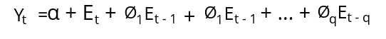
Here the error terms are the errors of the autoregressive models of the respective lags.
The mathematical equation of the ARIMA model
An ARIMA model is where you should make the time series at least once to make it stationary.
A stationary time series is one whose properties do not depend on the time at which the series is observed. Thus, time series with trends, or with seasonality, are not stationary — the trend and seasonality will affect the value of the time series at different times.
Stationarity and differencing | Forecasting – OTexts
We develop the ARIMA model’s equation by combining AR and MA equations.
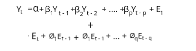
In other words, the predictive value of the ARIMA model is given by:
Y-pred = Constant + Linear combinations of lags of Y(up to p) + linear combinations of lagged forecast error(up to q).
What is stationary time series?
A stationary time series is one whose properties do not depend on the time at which the series is observed. Thus, time series with trends or seasonality are non-stationary because the trend and seasonality will affect the value of the time series at different times. On the other hand, a white noise series is stationary, as it does not matter when we observe it. It should look much the same at any point in time. A simple way to know a stationary times series is that the mean and variance of the stationary time series are constant over time.
The ARIMA model performs well on a stationary time series. So, if we get a non-stationary time series, we must convert it into stationery to train the ARIMA model. There are various ways to make a non-stationary time series into a stationary time series. The two most common ones are Differencing and Transforming. We will use both methods to transform a non-stationary time series into a stationary time series in the upcoming sections.
Steps of Building the ARIMA model
We will use the following steps to build the ARIMA model:
- Explore dataset
- Check if the dataset is non-stationary
- Apply either differencing or transformation methods to make time-series stationary
- Find the relevant values for
p,d, andq. - Train the model
- Evaluate the model and make predictions
Implementation of the ARIMA model using Python
Now we will implement the ARIMA model on the dataset, which is about the sales of Catfish. You can access the dataset from this link.
Before implementing the ARIMA model, ensure that you have installed the following Python modules.
- pandas
- numpy
- matplolib
You can use the pip command to install the required modules.
%pip install pandas
pip install numpy
pip install matplotlib
Once the installation is complete, we can move to the implementation part.
Importing and exploring the dataset
We will use the pandas’ module to import the data set and explore its features.
# importing the required module
import pandas as pd
# importing the dataset
df = pd.read_csv("catfish.csv")
# printing
df.head()
Output:
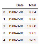
As you can see, there are two columns, one representing the data and the next one total catfish sales.
Now let us also see if there are any null values in our dataset.
# checking for null values
df.isnull().sum()
Output:
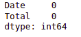
This shows that there are no null values in our dataset.
We will now visualize the dataset to see the overall trend of the time series dataset.
# importing the module
import matplotlib.pyplot as plt
# setting the size
plt.figure(figsize=(15,8))
# plotting the graph
plt.plot(df.Date, df.Total)
plt.show()
Output:
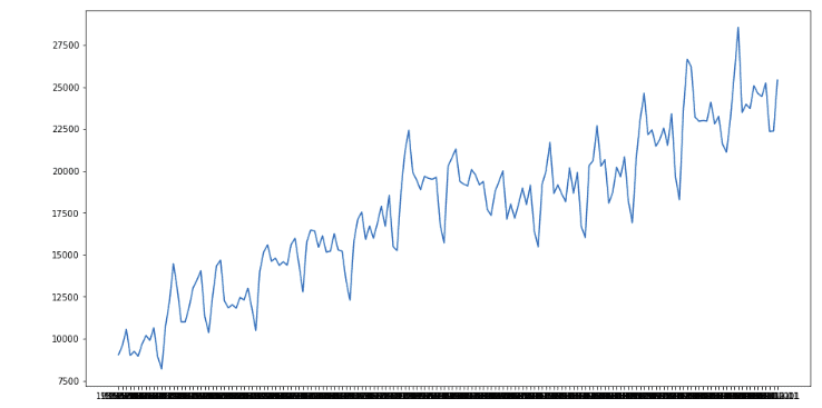
Now let’s go to the implementation of the ARIMA model.
Differencing time series to make it stationary
As we know that the ARIMA models take three parameter values p, q, and d, so before training the model, we must find the values for each of these terms. The d here represents the number of differencing it takes to stationary the time series. So, let us now apply the 1-st differencing to see if the time-series data becomes stationary.
# Importing the modules
from statsmodels.graphics.tsaplots import plot_acf, plot_pacf
# fixing the size
plt.rcParams.update({'figure.figsize':(9,7), 'figure.dpi':120})

# Original Series
fig, axes = plt.subplots(2, 2, sharex=True)
axes[0, 0].plot(df.Total); axes[0, 0].set_title('Original Series')
plot_acf(df.Total, ax=axes[0, 1])
# 1st Differencing to make stationary time series data
axes[1, 0].plot(df.Total.diff()); axes[1, 0].set_title('1st Order Differencing')
plot_acf(df.Total.diff().dropna(), ax=axes[1, 1])
plt.show()
plt.show()
Output:
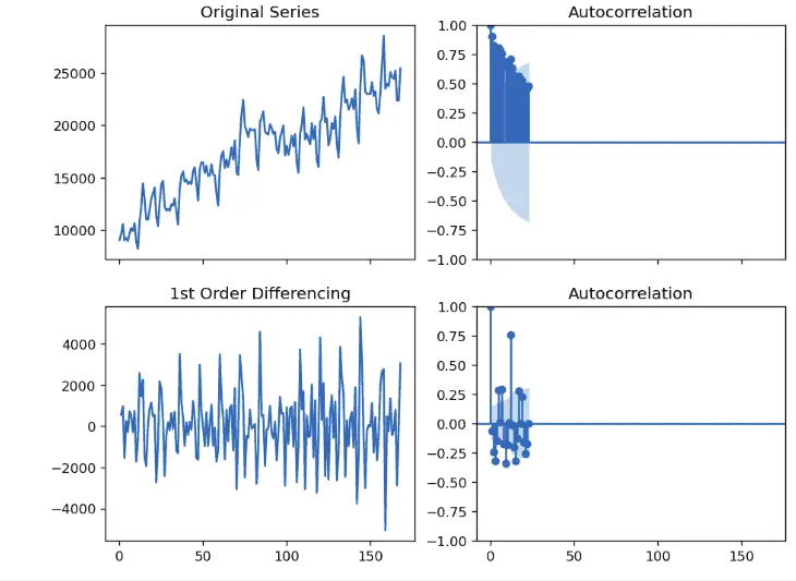
As we can see, the time series becomes nearly stationary in the first differencing. So, we will set the value of d equal to 1.
Finding the order of the AR model
As we know, the ARIMA model combines the AR and MA models. So, first, let us find the order of the AR model.
We will determine the required number of AR terms by inspecting the Partial Autocorrelation (PACF) plot. Partial autocorrelation can be imagined as the correlation between the series and its lag after excluding the contributions from the intermediate lags. In other words, partial autocorrelation is the relation between observed at two-time spots, given that we consider both observations to be correlated to the observations at other time spots. For example, today’s stock price can be correlated to the day before yesterday, and yesterday can also be the day before yesterday.
Let’s now plot the partial auto-correlation plot using Python:
#importing modules
from statsmodels.graphics.tsaplots import plot_acf, plot_pacf
# PACF plot of 1st differenced series
plt.rcParams.update({'figure.figsize':(9,3), 'figure.dpi':120})
# fixing the axis
fig, axes = plt.subplots(1, 2, sharex=True)
# plotting on differen axis
axes[0].plot(df.Total.diff()); axes[0].set_title('1st Differencing')
axes[1].set(ylim=(0,5))
# plotting partial autocorrelation function
plot_pacf(df.Total.diff().dropna(), ax=axes[1])
plt.show()
Output:
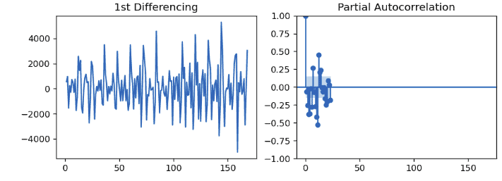
In the Partial autocorrelation plot, the light blue area shows the significant threshold value, and every vertical line indicates the PACF values at each time spot. So in the plot, only the vertical lines that exceed the light blue area are considered significant. We can see that PACF lag 1 is significant since it is well above the signature line. So, we will set the p value equal to 1.
Finding the order of the MA model
An ACF (autocorrelation function) is a correlation between the observations at the current time spot and those at previous time spots. Like how we looked at the PACF plot for the number of AR terms, we will look at the ACF plot for the number of MA terms. An MA term is simply the error of the lagged forecast.
Let’s now plot the ACF plot using Python for our dataset:
# setting the size
plt.rcParams.update({'figure.figsize':(9,3), 'figure.dpi':120})
#  fixing the subplots
fig, axes = plt.subplots(1, 2, sharex=True)
axes[0].plot(df.Total.diff()); axes[0].set_title('1st Differencing')
axes[1].set(ylim=(0,1.2))
# plotting the autocorrelation function
plot_acf(df.Total.diff().dropna(), ax=axes[1])
plt.show()
Output:
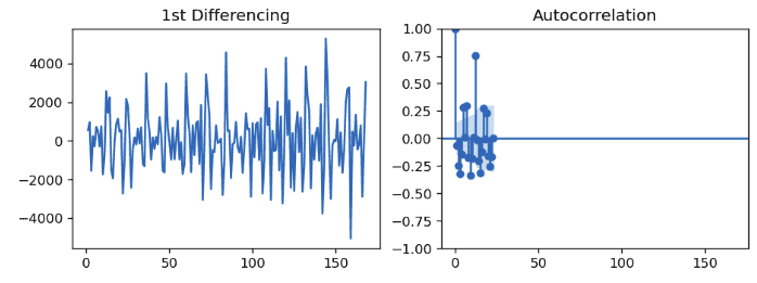
We can see that couple of lags are well above the signature line, but we will fix q to 1 one vertical line is quite significant in the plot.
Building ARIMA model
Now we have the values for p, q, and d, we can train the ARIMA model on the time series dataset.
# importing the ARIMA model
from statsmodels.tsa.arima_model import ARIMA
# 1,1,1 ( arima p d q )
model = ARIMA(df.Total, order=(1,1,1))
# Training arima modeling
model_fit = model.fit()
Once the training is complete, we can then plot the actual and the predicted value of the model using the plot_predict() method.
# arima model results
model_fit.plot_predict(dynamic=False)
plt.show()
Output:
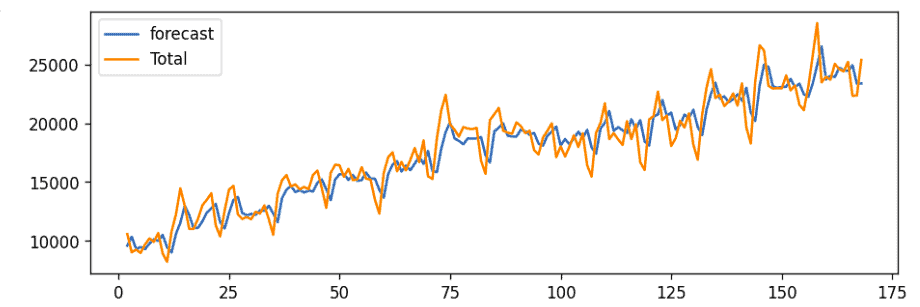
The blue line shows the predicted values, and the orange line shows the actual values. The prediction seems to follow the trend, and it seems to have a decent ARIMA model. But, we can’t say this is the best ARIMA model because we haven’t forecasted the future and compared the forecast with the actual performance.
Out-of-Time cross-validation
In Out-of-Time cross-validation, we move backward in time and forecast into the future. Then we can compare the forecast and the actual values to see how well the predictions are. For that purpose, we will create the training and testing dataset by splitting the time series into 2 contiguous parts in a reasonable proportion based on the time-frequency of the series.
Let’s first split the time series dataset into testing and training parts.
# Create Training and Test
train = df.Total[:130]
test = df.Total[130:]
Now we can use the training data to train and then use the testing part to evaluate the performance of the ARIMA model.
#  Build Model
model = ARIMA(train, order=(1, 1, 1))
fitted = model.fit()
# Forecast using 95% confidence interval
fc, se, conf = fitted.forecast(39, alpha=0.05)
# Make as pandas series
fc_series = pd.Series(fc, index=test.index)
lower_series = pd.Series(conf[:, 0], index=test.index)
upper_series = pd.Series(conf[:, 1], index=test.index)
# Plot
plt.figure(figsize=(12,5), dpi=100)
plt.plot(train, label='training')
plt.plot(test, label='actual')
plt.plot(fc_series, label='forecast')
plt.fill_between(lower_series.index, lower_series, upper_series, color='k', alpha=.15)
plt.title('Forecast vs Actuals')
plt.legend(loc='upper left', fontsize=8)
plt.show()
Output:
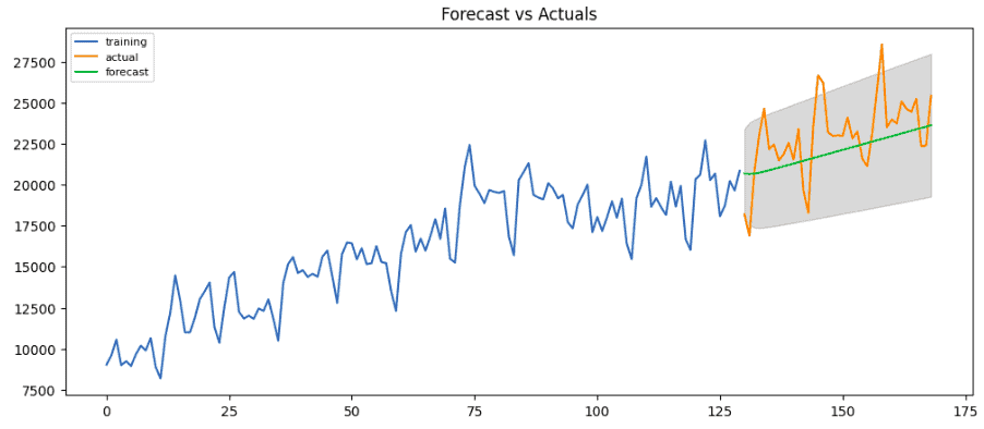
The green line shows the predicted values while the orange shows the actual values, and the grey region represents the confidence interval. We can see from the plot that the model has performed well.
Implementation of ARIMA on the non-stationary time series
Now we will explore important transformation methods to convert a non-stationary time series into a stationary time series. For that purpose, we will use a dataset about Air passengers. You can download the dataset from this link.
Importing and exploring the time series
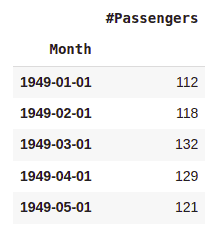
We will import the dataset and print out a few rows using the Pandas module.
#importing datatime
from datetime import datetime
# Importing the dataset
dataset = pd.read_csv('AirPassengers.csv')
#converting string to Pandas datatime
dataset['Month'] = pd.to_datetime(dataset['Month'],infer_datetime_format=True)
df = dataset.set_index(['Month'])
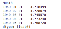
# printing
df.head(5)Output:
The next step is to see if there are any null values.
# checking for null values
df.isnull().sum()
Output:

As we can see, there are no null values. Now will plot the time series dataset.
# labeling
plt.xlabel('Date')
plt.ylabel('Number of air passengers')
# plotting
plt.plot(df)
plt.show
Output:

As we can see, the number of passengers had increased overall, but there were some fluctuations.
Check if the time series is stationary
As we already discussed, the easiest way to know if a time series is stationary is to check if its mean and standard deviation is constant. If both are constant over time, the time series is stationary.
So, let us find the mean and standard deviation and plot them.
#Determine rolling statistics
rolmean = df.rolling(window=12).mean()
rolstd = df.rolling(window=12).std()
Notice that the window size is 12 denotes 12 months which gives the rolling mean yearly.
Now we will plot the mean and standard deviation.
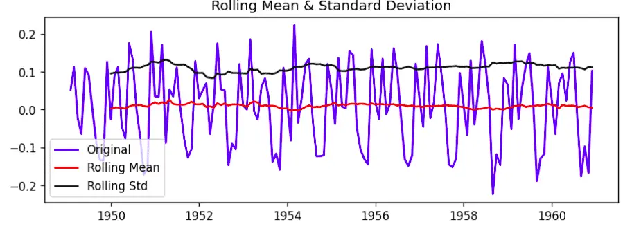
#Plot rolling statistics
orig = plt.plot(df, color='blue', label='Original')
mean = plt.plot(rolmean, color='red', label='Rolling Mean')
std = plt.plot(rolstd, color='black', label='Rolling Std')
# labeling
plt.legend(loc='best')
plt.title('Rolling Mean & Standard Deviation')
plt.show()
Output:
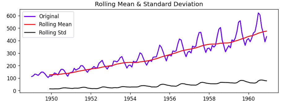
Notice that the standard deviation is nearly constant, but the mean is not, suggesting that the time series is not stationary.
Data transformation to make time-series data stationary
There are many ways to make a non-stationary time series stationary. For example, using log, square, square root, cube, cube root, and many other useful methods. Here we will discuss some of these methods to transform our time series into stationery.
Log scale transformation
Log transformation is a data transformation method that replaces each variable x with a log(x). Let us now use log scale transformation and see if it can transform our dataset into a stationary dataset.
# importing the module
import numpy as np

#Estimating trend
logScale = np.log(df)
#The below transformation is required to make series stationary
movingAverage = logScale.rolling(window=12).mean()
movingSTD = logScale.rolling(window=12).std()
# plotting the graph
plt.plot(logScale)
plt.plot(movingAverage, color='red')
plt.show()
Output:
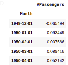
Now we have the log(x) values of the time series. So, to make it stationary, we can create a function that subtracts the rolling mean and the mean of the log scale (above one) so that the resulting mean will be stationary.
We will transform our dataset into a new dataset that will differentiate between the rolling and log scale mean.
# Trasformed dataset
log_transformed = logScale - movingAverage
log_transformed.head(12)
#Remove NAN values
log_transformed.dropna(inplace=True)
# printing heading of dataset
log_transformed.head()
Output:
First, find the transformed time series dataset’s rolling mean and standard deviation and then plot them.
#Determine rolling statistics
movingAverage = log_transformed.rolling(window=12).mean()
movingSTD = log_transformed.rolling(window=12).std()

#Plot rolling statistics for the transformed dataset
orig = plt.plot(log_transformed, color='blue', label='Original')
mean = plt.plot(movingAverage, color='red', label='Rolling Mean')
std = plt.plot(movingSTD, color='black', label='Rolling Std')
# plotting stationary time series data
plt.legend(loc='best')
plt.title('Rolling Mean & Standard Deviation')
plt.show()
Output:
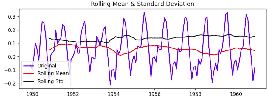
Notice that the mean and standard deviation are nearly constant, suggesting that the transformed time series data is now stationary.
Timeshift transformation
We will use the time shift transformation to transform non-stationary time series into stationary data.
Let us first plot the transform data using timeshift transformation.
# transforming the dataset
Shifting = logScale - logScale.shift()
# plotting
plt.plot(Shifting)
plt.show()
Output:
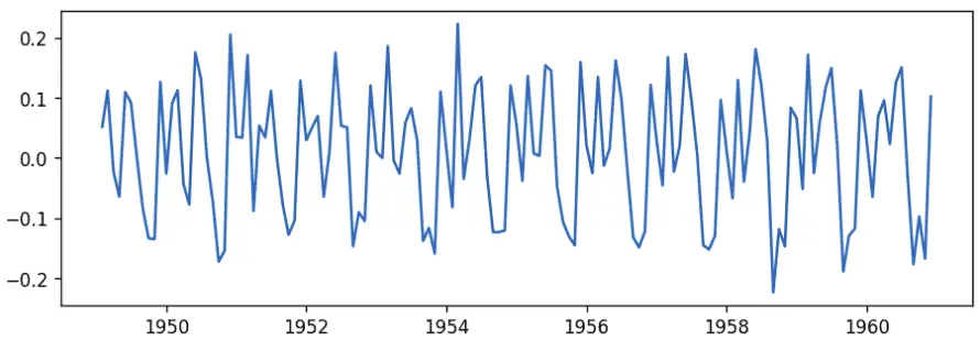
As you can see that there is no trend now. Let us also plot the transformed data’s rolling mean and standard deviation.
#Determine rolling statistics
movingAverage = Shifting.rolling(window=12).mean()
movingSTD = Shifting.rolling(window=12).std()

#Plot rolling statistics for the transformed dataset
orig = plt.plot(Shifting, color='blue', label='Original')
mean = plt.plot(movingAverage, color='red', label='Rolling Mean')
std = plt.plot(movingSTD, color='black', label='Rolling Std')
# Labeling
plt.legend(loc='best')
plt.title('Rolling Mean & Standard Deviation')
plt.show()
Output:
As you can see that the rolling standard deviation and mean are nearly constant, which shows that the dataset is now stationary.
Similarly, you can use any other method to transform the time series into stationery.
Building ARIMA Model
We used two different ways to transform the data into a stationary dataset. This section will describe the log scale transformed time series to train the ARIMA model.
As we explained earlier, you can use ACF and PACF methods to determine the optimum value for p and q. In this section, we will not spend time again finding optimum ACF and PACF values.
# 2, 1, 2 (arima p d q )
model = ARIMA(logScale, order=(2,1,2))
# fiting the model
results_ARIMA = model.fit()
# plotting the results
plt.plot(Shifting)
plt.plot(results_ARIMA.fittedvalues, color='red')
plt.show()
Output:
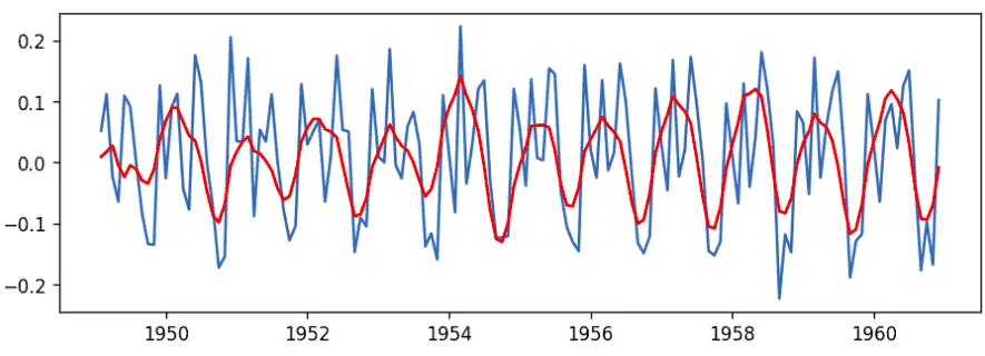
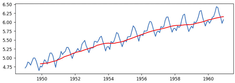
As you can see, the best-fitted line by the model is the orange one. But this visualization is on the transformed data, so let us again change the data back to its original form.
Predictions and reverse transformation
Now let us make predictions and reverse the transformation to get the original dataset.
# making predictions
predictions_ARIMA = pd.Series(results_ARIMA.fittedvalues, copy=True)
#Convert to cumulative sum
predictions_ARIMA_cumsum = predictions_ARIMA.cumsum()
# reversing the transformation to original data
predictions_ARIMA_log = pd.Series(logScale['#Passengers'].iloc[0], index=logScale.index)
predictions_ARIMA_log = predictions_ARIMA_log.add(predictions_ARIMA_cumsum, fill_value=0)
# printing heading
predictions_ARIMA_log.head()
Output:
These are the values of the best-fitted line of the model. Let us visualize the original dataset and these predictions to evaluate our model.
# Inverse of log is exp
predictions_ARIMA = np.exp(predictions_ARIMA_log)
# plotting actual values
plt.plot(df)
# plotting predictions
plt.plot(predictions_ARIMA)
plt.show()
Output:
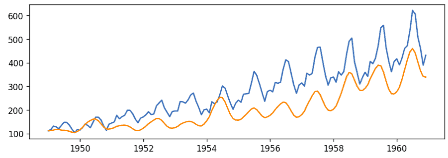
The above graph shows that the model has learned the trend and has predicted pretty well.
As our model has been trained and learned the patterns. We can use the plot_predict() function to make predictions for the future. We know we had data for the last 12 years, so based on the given dataset, let us predict the number of passengers for five years with a 90% confidence interval.
# predict future points ( for 5 years)
results_ARIMA.plot_predict(1, 204)
Output:
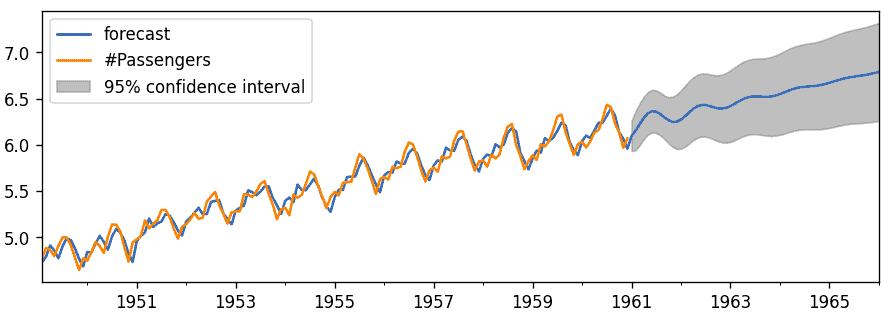
The blue line shows the predictions, while the grey region represents the confidence interval.
Summary
ARIMA is a class of statistical models for analyzing and forecasting time series data. It is a combination of AR and MA models. In this article, we covered the ARIMA model in detail. We also learn to convert non-stationary time series into stationary using various methods.
If you’d like to dive deeper, we suggest you check out one of the most popular Udemy courses – Python for Time Series Data Analysis.
