Facebook Prophet: A Simple Algorithm for Time-Series Data
Time series data is data that is recorded over consistent intervals of time. Sometimes, it is difficult and frustrating to work with such data. As most of the algorithms that generate models for time series data can be quite finicky and hard to tune. In this article, we will discuss Facebook Prophet which is one of the simplest algorithms to deal with time-series data. We’ll cover the Facebook Prophet algorithm and apply it to time-series datasets to explore its important parameters.
Table of contents
We assume that you have basic knowledge of Machine Learning and various key phrases that are used in machine learning, for example, models, training the model, predictions, etc. We also assume that you have knowledge of the time series data and other datasets because in this article we will be using time-series datasets to make predictions.
Key features of the Facebook Prophet
The following are the key features of the Facebook Prophet that make it a unique time series predicting algorithm.
- The Facebook Prophet is accurate and fast.
- Prophet allows adjustment of parameters and customized seasonality components which may improve the forecasts.
- Prophet can also handle outliers and handles other data issues by itself.
- The holiday function allows Prophet to adjust forecasting when a holiday or major event may change the forecast.
- It can detect the change points automatically.
Explanation of Facebook Prophet
In 2017, researchers at Facebook published a paper called, “Forecasting at Scale” which introduced the project Facebook Prophet. It is an open-source algorithm for generating time-series models that uses a few old ideas with some new twists. It is particularly good at modeling time series that have multiple seasonalities. Seasonality is a characteristic of a time series in which the data experiences regular and predictable changes that recur every calendar year. Or in other words, any predictable fluctuation or pattern that recurs or repeats over a one-year period is said to be seasonal.
In general, the Facebook Prophet is the sum of three different functions along with an error term as shown below:
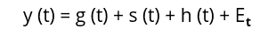
y(t) – is the output value.
g(t) – is a piecewise linear or logistic growth curve for modeling non-periodic changes in time series.
s(t) – is periodic changes (e.g. weekly/yearly seasonality).
h(t) – It is the effects of holidays (user-provided) with irregular schedules
Et – is an error term that accounts for any unusual changes not accommodated by the model.
Now let’s dive into each of these functions to understand what they actually represent.
The Growth function
The Facebook Prophet provides three options for growth function which are represented by g(t) in the main equation. It can either be linear, logistic, or flat depending on the dataset. In general, the growth function models the overall trend of the data.
Linear growth is the default setting for the Facebook Prophet. It uses a set of piecewise linear equations with differing slopes between change points.
If the time series has a cap or a floor in which the values and the modeling becomes saturated and can’t surpass a maximum or minimum value, then we use logistic regression as our growth function.
The flat is used as a growth function if trend there is no growth over time. If the growth function is flat, it will be a constant value.
The seasonality and holiday function
The seasonality function is represented by s(t) and the holiday function is represented by h(t) in the main equation. As we discussed seasonality refers to the presence of variations that occur at certain regular intervals either on a weekly basis, monthly basis, or even quarterly. Various factors may cause seasonality – like a vacation, weather, and holidays. For example, people buy a lot of stuff for Christmas, so the sales around Christmas days are high. Prophet allows the analyst to provide a custom list of past and future events. A window around such days is considered separately and additional parameters are fitted to the model to understand the effects of holidays and events.
Implementation of Prophet on a time series dataset
We will now implement the Prophet algorithm on a time series dataset to predict sales in the future. The dataset about the sales of catfish from 1986 to 2001. You can access the dataset from this link.
Before going into the implementation part, ensure you have installed the following required Python modules.
- sklearn
- prophet
- pandas
- numpy
- matplotlib
You can install the given modules by running the following command in the cell of the Jupyter notebook.
%pip install prophet
pip install sklearn
pip install pandas
pip install numpy
pip install matplotlib
Once the installation is complete, you can go to the implementation part.
Importing and exploring the dataset
We will use pandas to import the dataset. The dataset contains two columns, one showing the date and another column showing the total sale.
# importing pandas
import pandas as pd
# importing forecasting dataset
catfish = pd.read_csv('catfish.csv')
# business forecasts heading
catfish.head()
Output:

As the input to Prophet is always a data frame with two columns:
- The datestamp column should be of a format expected by Pandas, ideally YYYY-MM-DD for a date or YYYY-MM-DD HH:MM: SS for a timestamp.
- The
ycolumn must be numeric and represents the measurement we wish to forecast. So, our dataset is ideal data for the Prophet algorithm.
We will use info() method of pandas to get more information about the data.
# info about forecasting time series data
catfish.info()
Output:
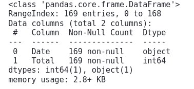
This shows that there are a total of 169 observations with two columns and there are no missing observations.
Let us now plot the dataset on a graph to see more clearly how the data is arranged and distributed.
# importing matplotlib module
import matplotlib.pyplot as plt
# setting the size of the plot
plt.figure(figsize=(15, 8))
# plotting forecast sales
plt.plot(catfish.Date, catfish.Total)
plt.show()
Output:
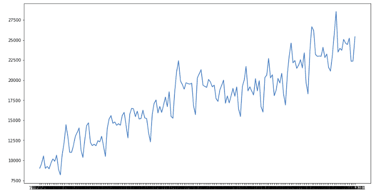
Notice that the sales are increasing with a trend and there few specific times, where the sale is drastically decrease and then increase. We will visualize these trends using the Prophet algorithm.
Training the Prophet model
Before using the dataset for the training, let us first rename the columns. We will assign ds to the Date column and y to the Sales column.
# python code to rename the columns
catfish.rename(columns={'Date':'ds','Total':'y'},inplace=True)
Now let us use the dataset to train the model. We first need to import the Prophet and then initialize it. We will assign a confidence interval of 95%. A confidence interval is a range of values so defined that there is a specified probability that the value of a parameter lies within it.
# importing python time series packages
from prophet import Prophet
# initialiazing the model with 95% confidence interval
model = Prophet(interval_width= 0.95)
# train model
model.fit(catfish)
Once the training of the model is complete, we can go for the forecasting.
Forecasting time series data
Predictions are made on a data frame with a column ds containing the dates for which a prediction is to be made. The algorithm provides a make_future_dataframe() method to make predictions for the future. Let us now apply this method to get future dates for predictions.
# forecasting for future
future = model.make_future_dataframe(periods=80, freq='M')
The future variable just contains dates starting from 1986 which was the starting date in the training dataset till specified periods. So, if we print out the first few rows, it will be similar to the original dataset.
# forecating head
future.head()
Output:
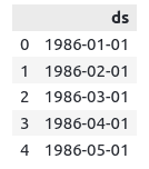
Note that the starting date is the same as that of the training dataset. But if we will print the tail of the future, it will have more dates than our original dataset.
# tail of forecasting dates
future.tail()
Output:
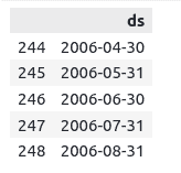
Notice that there are a total of 248 rows and the dates are up to 2006 while in the original dataset, there were only 169 rows as shown below:
# total dates
catfish.tail()
Output:
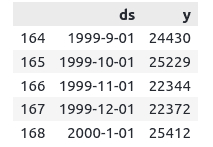
As you can see that the original dataset also contains the output values as well while the future variable has only dates. We will now provide these dates to the trained model which will make forecast predictions.
Visualizing the forecast predictions
Let’s make predictions by using only dates.
# forecast predictions
forecast = model.predict(future)
Let’s again print the predictions of the model using head() method.
# Prophet's prediction head
forecast.head()
Output:
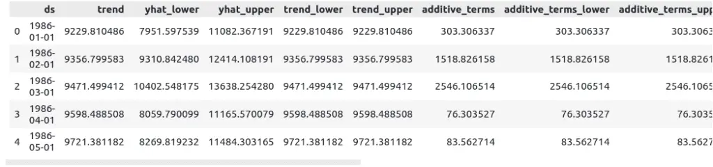
The predicted dataset contains a lot of information about the predictions and trained model. It shows the overall trend, upper limit, lower limit, yearly trend, weekly trend, and many more. But our main focus is the very last column of the dataset which contains the predicted values of the model.
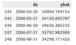
# showing the predictions
forecast[['ds', 'yhat']].tail()
Output:
Let us now visualize the predictions along with the actual values and the limits (upper and lower limits).
# visualizing the forecat predictions
fig1 = model.plot(forecast)
Output:
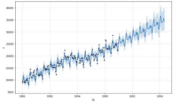
The black dotted points show the actual data points. The blue line shows the predictions of the model and the light-blue is the upper limit and lower limit. The graph shows that Prophet performs very well. It has learned the trends in the data points and predicted the future based on these trends.
One of the cool things about the model is that we can also visualize the trends based on the weekly seasonal component, monthly seasonal component, and yearly seasonal component based on the training dataset. For example in our case, we can visualize the monthly and yearly trends based on the training of the model.
# weekly seasonality and yearly seasonality
fig2 = model.plot_components(forecast)
Output:
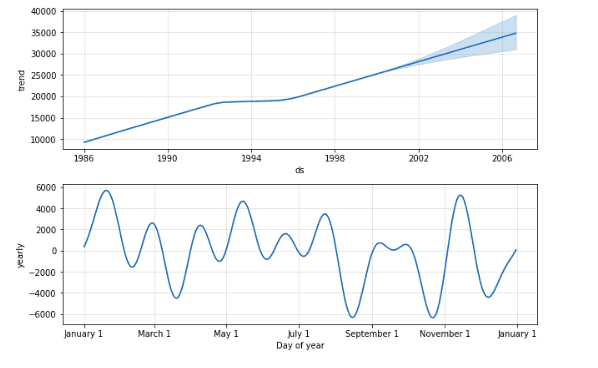
The above plots are known as component plots. The first plot is the yearly seasonal component plot. It shows that the overall trend in the sales is increasing except from 1993-1995, where the sales were nearly constant. After 2001, the plot shows the predicted values for sales with upper and lower limit intervals. While the second plot is the monthly seasonal component plot. It shows that in August and October, the sales are very low and have high sales in January and November moths,
Changepoint Detection in a Time series data
You may have noticed that the time series data have some abrupt changes in their trajectories. By default, Prophet will automatically detect these changepoints and will allow the trend to adapt appropriately. Let us now visualize those changepoints that were automatically detected by the Prophet model.
# import the ploting module
from prophet.plot import add_changepoints_to_plot
# creating plot
fig = model.plot(forecast)
# completely automatic forecasting techniques
change_points = add_changepoints_to_plot(fig.gca(), model, forecast)
Output:
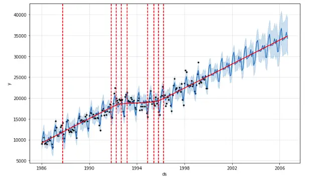
The vertical lines in the plot indicate the potential changepoints detected by the model.
By default, change points are only inferred for the first 80% of the time series in order to have plenty of runway for projecting the trend-forward and to avoid overfitting fluctuations at the end of the time series. We can change this value by using changepoint_range parameter’s value. For example, let us visualize the change points by specifying the changpoint_range to be the first 50% of the dataset.
# initializng the model with 50% of the changepoint range
model = Prophet(changepoint_range=0.5)
# train model
model.fit(catfish)
# forecasting for future
future = model.make_future_dataframe(periods=80, freq='M')
# forecast predictions
forecast = model.predict(future)
# creating plot
fig = model.plot(forecast)
# completely automatic time series analysis
change_points = add_changepoints_to_plot(fig.gca(), model, forecast)
Output:
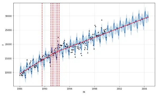
Notice that now the model has detected the change points only within the first 50% of the dataset.
Predicting Bitcoin price using Facebook Prophet
Now we will take a real dataset and use the Prophet to make predictions. We will take the data about the price of Bitcoin for the last year and make predictions for the future. You can access the dataset from this link.
For those who don’t know about Bitcoin, it is a digital currency that operates free of any central control or the oversight of banks or governments. Instead, it relies on peer-to-peer software and cryptography. You can read more about Bitcoin from their official website.
Exploring the dataset
Let’s first import the dataset and print out a few rows using the Pandas module.
# importing BITCOIN data
BTC = pd.read_csv('BTC_Three_years.csv')
# printing the heading
BTC.head()
Output:

Note that the dataset contains more information (opening, high, low, and closing prices in USD dollar). We only need two columns to train the model. So, we will use the Date and the closing price of Bitcoin and will remove all other columns.
# Removing the columns
BTC.drop('Open', axis=1, inplace=True)
BTC.drop('High', axis=1, inplace=True)
BTC.drop('Low', axis=1, inplace=True)
Let us now use the pandas info() method to get more information about the dataset.
# Info method
BTC.info()
Output:
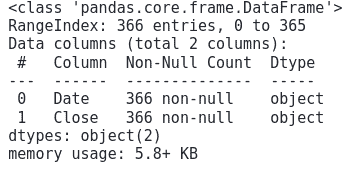
This shows that there are a total of 366 observations and there are no missing data. Also notice that the columns are of object data type. We need to convert them into Date format and float data type, before using them for training the model. But before converting the Close column to floating, we need to remove the commas.
# removing the commas
BTC['Close']=BTC['Close'].str.replace(',','')
We will now convert the columns into Date and float data types.
# convert the 'Date' column to datetime format
BTC['Date']= pd.to_datetime(BTC['Date'])
BTC["Close"] = pd.to_numeric(BTC["Close"], downcast="float")
As we know the algorithm expects the column names to be ds and y. So, we will rename the column names.
# Renaming the columns names
BTC.rename(columns = {'Date':'ds', 'Close':'y'}, inplace = True)
Let us visualize the data to see how the closing price of Bitcoin changes over one year of time.
# setting the size
plt.figure(figsize=(15, 8))
# plotting the scatter plot
plt.scatter(BTC.ds, BTC.y)
plt.show()
Output:
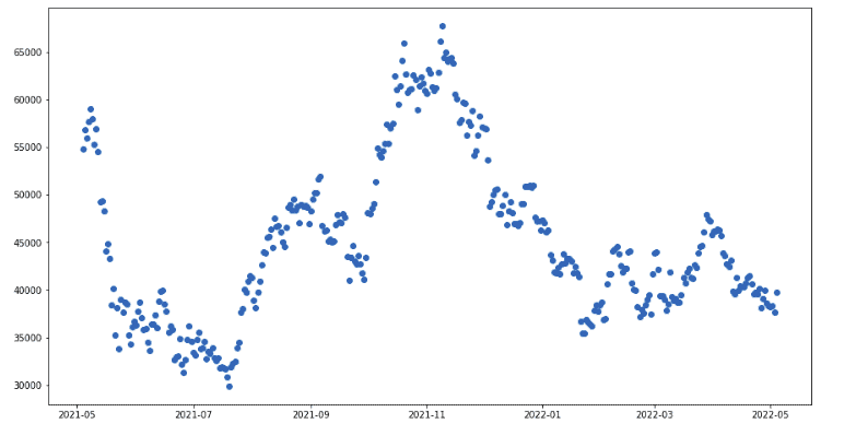
The plot shows there is a big variation in the closing price of Bitcoin over one year.
Training the model with linear growth
As we know by default the growth in the Prophet is linear. First, we will train the model using the default growth and then make predictions.
# initialiazing the model with 80% confidence interval
model = Prophet(interval_width=0.8)
# business forecast tasks training
model.fit(BTC)
Once the training is complete, we can make input values ( dates ) for future predictions.
# historical data and future data
future = model.make_future_dataframe(periods=2, freq='M')
We created data for the next two months.
Let us now use this dataset to make predictions for the future using the model.
# forecast predictions
forecast = model.predict(future)
Once the predictions are complete, we can visualize the future predicted price of the Bitcoin by the model.
# visualizing time series analysis
fig1 = model.plot(forecast)
Output:
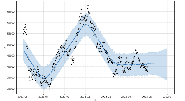
The predicted line ( blue) suggests that the price of Bitcoin will remain nearly constant in the next couple of months. While the light-blue area is the confidence interval ( 80%).
Let us now visualize the weekly seasonality and monthly seasonality of the Bitcoin for the last year.
# weekly and monthly time series analysis
fig2 = model.plot_components(forecast)
Output:
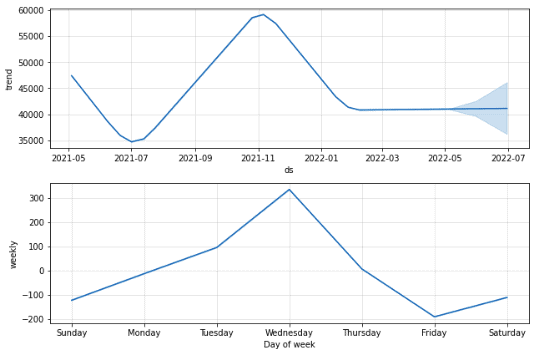
The first plot shows the overall trend for the last year. While the second plot is very interesting. It shows that the price usually increases on Wednesday and then decreases till Friday. That means if you buy Bitcoins on Friday and sell them on Wednesday, you can earn a lot of profits.
Training the model with logistic growth
Prophet allows us to make forecasts using a logistic growth trend model, with a specified carrying capacity. A carrying capacity is usually some maximum achievable point. The important things about the carrying capacity are that it can be specified for every row in the data frame or it can also be constant based on data. If the market size is growing, then the carrying capacity can be in an increasing sequence.
In our case, we will fix the carrying capacity to a constant value, because the prices last year are increasing and decreasing at the same time. There is no specific trend.
# carrying capacity
BTC['cap'] = 80000
We fixed the carrying capacity to 80000 USD dollars.
Let us now train the model on the dataset.
# confidence interval of 50%
model_logistic = Prophet(growth='logistic', interval_width=0.5)
# fitting the model
model_logistic.fit(BTC)
Once the training is complete, we can make predictions for the future. To create a future dataset, we also need to specify the carrying capacity.
# forecasting for future
future = model_logistic.make_future_dataframe(periods=2, freq='M')
# carrying capacity
future['cap'] = 80000
# predictions
forecast_logistic = model_logistic.predict(future)
Once the predictions are complete, we can visualize the predictions for an upcoming couple of months.
# visualizing the forecat predictions
fig1 = model.plot(forecast_logistic)
Output:

The plot shows that the price of Bitcoin is likely to decrease in the upcoming couple of months.
Let’s again visualize the components of the logistic model as well.
# weekly weekly observations and monthly time series analysis
fig2 = model.plot_components(forecast_logistic)
Output:

The first plot shows that for the last year, the price increased in the beginning and then started to decrease. At the same time, the second plot shows similar results to the linear model. It shows the price of Bitcoin increases from Sunday to Wednesday and then starts decreasing till Friday. So, if you buy Bitcoins on Friday and sell them on Wednesday, you can earn a lot of profit.
Summary
In this article, we learn about the key features of the Prophet, an open-source forecasting tool in Python and R. We used Python language to apply it to various datasets and learn how to interpret the results.
