Implementation of Logistic Regression using Python
Machine Learning is the study of computer algorithms that can automatically improve through experience and using data. ML consists of three main categories; Supervised learning, Unsupervised Learning, and Reinforcement Learning. Logistic Regression belongs to Supervised learning algorithms that predict the categorical dependent output variable using a given set of independent input variables. This article will use Python to cover Logistic Regression, its implementation, and performance evaluation.
Table of contents
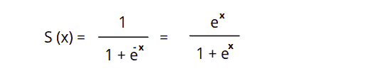
Logistic Regression is very similar to Linear Regression, but instead of solving regression problems, it is used to solve classification purposes. In Logistic Regression, we use an S-shaped logistic function (sigmoid) instead of a simple regression function. In the upcoming sections, we cover the mathematical calculations behind Logistic Regression that will help us distinguish it from Linear Regression.
Overview of Logistic Regression Algorithm
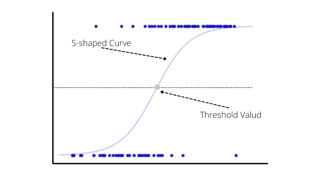
Logistic Regression is an important Machine Learning algorithm because it can provide probability and classify new data using continuous and discrete datasets. When the dependent variable (output) is categorical, you must use Logistic Regression. The Logistic Regression is based on an S-shaped logistic function instead of a linear line. The curve from the logistic function indicates the probability of an item belonging to one or category or class.
The following graphs show the predictive model of the Logistic Regression algorithm:
Different types of Logistic Regression depend on the classification data type.
- Binary Logistic Regression: The target variable has only two possible outcomes: Spam or Not Spam, Cancer or No Cancer.
- Multinomial Logistic Regression: The target variable has three or more nominal categories, such as predicting the type of disease or the age of a person.
- Ordinal Logistic Regression is used in cases when the target variable is ordinal. The categories are ordered meaningfully in this type, and each has quantitative significance. Moreover, the target variable has more than two categories. For example, the grades obtained on an exam have categories that have quantitative significance, and they are ordered.
Logistic Regression uses the sigmoid function, which maps predicted values to probabilities. It maps any real value into another value between 0 and 1. In Logistic Regression, we use the threshold value, which defines the probability of either 0 or 1. Such values above the threshold value tend to be 1, and a value below the threshold value tends to be 0.
Binary or Binomial Regression is the basic type of Logistic Regression in which the target or dependent variable can only be one of two types: 1 or 0. It allows us to model a relationship between a binary/binomial target variable and several predictor variables.
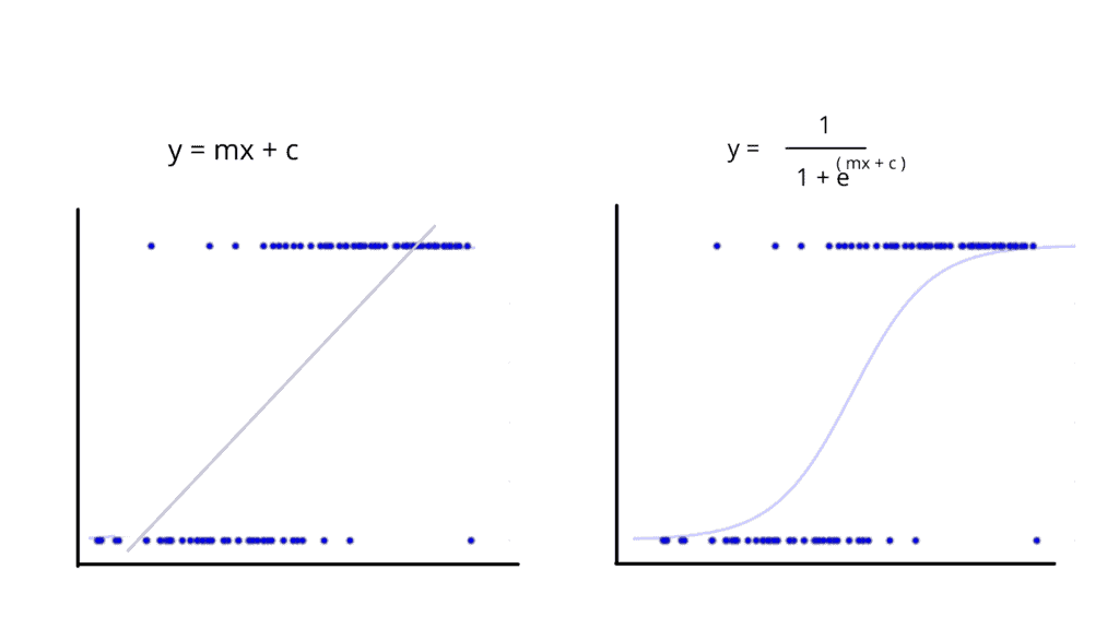
For some datasets (left plot below), the linear function is not excellently classifying the dataset items (dots). The Logistic Regression sigmoid function helps to fit the dataset better, and that’s the primary reason for using it.
Linear Regression vs. Logistic Regression
Here’s a list of primary differences betweenLinear and Logistic Regression:
| Feature | Linear regression | Logistic regression |
|---|---|---|
| Purpose | A supervised learning algorithm for solving regression problems | A supervised learning algorithm primarily used for classification problems |
| Types of problems to solve | Predicting the continuous dependent value of output variable based on independent variables, for example, the price of the house based on house parameters | Binary classification or separation of discreet dependent values with the help of independent variables, for example, predict whether a political candidate will win or lose an election or whether a product review is positive or negative |
| Type of output variable | Continuous value, for example, a value of age, height, time, price, salary, etc | A decimal value between 0 and 1 |
| Output function | Linear function predicts the output value or variable | An s-curve (sigmoid) function classifies the output variables |
| Accuracy estimation method | Ordinary Least Squares (OLS) | Maximum Likelihood Estimation (MLE) |
| Dependent/independent variables relationship | Linear | Not required |
| Collinearity (correlation between independent variables) | Allowed | Not allowed |
| Applications example | Stocks forecasting, item price prediction | General and text classification, image processing |
Assumptions of Logistic Regression
Logistic regression makes several assumptions:
- Binary outcome: The dependent variable must be dichotomous, meaning it has only two possible outcomes.
- Independence of observations: The observations must be independent of each other.
- Linearity in the logit: The logit transformation of the dependent variable must be a linear combination of the independent variables.
- No multicollinearity: The independent variables must not be highly correlated.
- Large sample size: The sample size should be large enough to avoid problems with statistical significance.
- No omitted variable bias: All important independent variables should be included in the model.
It’s important to note that these assumptions should be checked and confirmed before fitting the logistic regression model to ensure accurate and reliable results.
Implementing Logistic Regression using Python
Once we have a basic understanding of the Logistic Regression and maths used in the model’s training, let’s implement the Logistic Regression algorithm in Python step by step.
First, we must ensure that we have installed the following modules on our Jupyter notebook, which we will use in the upcoming sections. You can install them using the pip command in Jupyter Notebook cell:
%pip install numpy
%pip install sklearn
%pip install pandas
%pip install matplotlib
%pip install seaborn
Once these modules are installed successfully, we will go to the implementation part.
We will use the following steps to create our model and evaluate it:
- Data pre-processing
- Fitting Logistic Regression to the Training set
- Predicting the test result
- Test accuracy of the result (confusion matrix)
- Visualizing the result
Pre-processing dataset for Logistic regression
We will use a sample binary dataset to implement the Logistic Regression algorithm that contains information about various users obtained from social networking sites (you can download the data set from here).
Let’s imagine that the car-making company has launched a new SUV and wants to understand how many users from their internally collected dataset potentially wish to purchase the vehicle. The input or independent variables are the person’s age and salary.
To solve this business problem, we need to import all required modules and the dataset:
# importing the libraries
import pandas as pd
# importing the dataset
dataset = pd.read_csv('LogisticRegressionDAta.csv')
# printing dataset
print(dataset)
Output:
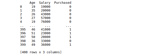
Note: two independent variables determine whether the person had purchased the car or not.
The next step is to store independent features and the output class in different variables.
# split the data into inputs and outputs
X = dataset.iloc[:, [0,1]].values
y = dataset.iloc[:, 2].values
The X variable will keep all independent features values (Age and Salary), and the y variable will hold the Purchase information (output).
Let’s visualize the dataset to see how many people purchased the car and how many did not. This information will help us see whether our data is balanced.
Here’s a good article that describes Unbalanced Datasets & What To Do About Them.
# importing the required modules for data visualization
import matplotlib.pyplot as plt
import chart_studio.plotly as py
import plotly.graph_objects as go
import plotly.offline as pyoff
# counting the total output data from purchased column
target_balance = dataset['Purchased'].value_counts().reset_index()
# dividing the output classes into two sections
target_class = go.Bar(
    name = 'Target Balance',
    x = ['Not-Purchased', 'Purchased'],
    y = target_balance['Purchased']
)
# ploting the output classes
fig = go.Figure(target_class)
pyoff.iplot(fig)
Output:

We need to have roughly the same number of examples for each output class for the balanced dataset. Out chart shows that the data is slightly unbalanced. There are several techniques that you can use to solve this problem. To simplify our example, we’ll continue with the existing dataset without any changes.
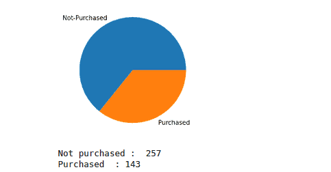
The pie chart can help visualize this better:
# importing numpy
import numpy as np
# creating variables
class_one = 0
class_two = 0
# for loop to itreate through the output class
for i in y:
    if i ==0:
        class_one+=1
    else:
        class_two+=1
# creating numpy arry
values = np.array([class_one, class_two])
label = ["Not-Purchased", "Purchased"]
# ploting the graph
plt.pie(values, labels = label)
plt.show()
# printing the results
print("Not purchased : ", class_one)
print("Purchased  :", class_two)
Output:
Training and testing the Logistic Regression model
The next step is to split our dataset into training and testing parts to train our model and then use the testing data to evaluate the model’s performance.
# training and testing data
from sklearn.model_selection import train_test_split
# assign test data size 20%
X_train, X_test, y_train, y_test =train_test_split(X, y, test_size= 0.2, random_state=0)
We’ll use 80% of the data for training and the remaining 20% for testing purposes.
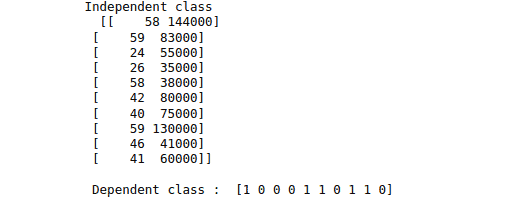
We’re storing Independent and dependent variables in the X_train and y_train variables for training and in X_test and y_test for testing.
print("Independent class \n " , X_train[:10])
print("\n Dependent class : ",y_train[:10])
Output:
Now, let’s apply the scaling method to the independent data so that the outliers would not affect the predicting class.
# importing StandardScaler
from sklearn.preprocessing import StandardScaler
# scalling the input data
sc_X = StandardScaler()
X_train = sc_X.fit_transform(X_train)
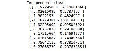
X_test = sc_X.fit_transform(X_test)If we print the X_train data now, it will be scaled in a small and specific range. For example, see below:
print("Independent class\n", X_train[:10])Output:
Now, let’s provide the scaled training dataset to our model and train it using the Logistic regression model.
# importing the logistic regression from sklearn module
from sklearn.linear_model import LogisticRegression
# fitting Logistic Regression to the training set
classifier= LogisticRegression()
classifier.fit(X_train, y_train)
Once the model’s training is complete, we can predict the output by providing the sample data point.
# Predicting a value
predicted_value = classifier.predict([[0.234, 1.2232]])
# printing the value
print(predicted_value)
Output:

Our model predicted that the customer with provided input data (Age, Salary) would buy the car, but we don’t know how accurate this prediction is yet.
To see the accuracy of the model’s prediction, we need to test the model by providing the testing dataset.
# testing the model
y_pred = classifier.predict(X_test)
# importing accuracy score
from sklearn.metrics import accuracy_score
# printing the accuracy of the model
print(accuracy_score(y_test, y_pred))
Output:

The output shows that the model’s accuracy is 88%, which is pretty good.
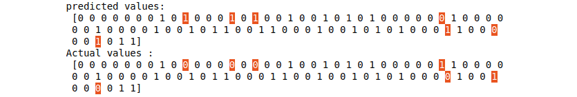
We can also print the predicted and actual values to see the difference.
# printing
print("predicted values:\n", y_pred)
print("Actual values :\n", y_test)
Output:
Visualizing training dataset
Let’s visualize the training set of our model. We will use ListedColormap class of the matplotlib module. We will create two new variables x_set and y_set to replace x_train and y_train. After that, we will use the nm.meshgrid command to create a rectangular grid, which ranges from -1 to 1. The pixel points we have taken will be of 0.01 resolution. We will use the mtp.contourf method to paint red and yellow regions. The classifier.predict method allows showing the predicted data points predicted by the classifier.
# importing modules
import numpy as np
from matplotlib.colors import ListedColormap
# seting x_train and y_train
x_set, y_set = X_train, y_train
x1, x2 = np.meshgrid(np.arange(start=x_set[:, 0].min()-1, stop = x_set[:, 0].max()+1, step=0.01),
np.arange(start=x_set[:, 1].min()-1, stop=x_set[:, 1].max()+1, step=0.01))
# ploting
plt.contourf(x1, x2, classifier.predict(np.array([x1.ravel(), x2.ravel()]).T).reshape(x1.shape),
alpha = 0.75, cmap = ListedColormap(('red','yellow')))
plt.xlim(x1.min(), x1.max())
plt.ylim(x2.min(), x2.max())
# for loop to iterate the data
for i, j in enumerate(np.unique(y_set)):
    plt.scatter(x_set[y_set == j, 0], x_set[y_set == j, 1],
        c = ListedColormap(('black', 'green'))(i), label = j)

# labeling the graph
plt.title('Logistic Regression (Training set)')
plt.xlabel('Age')
plt.ylabel('Estimated Salary')
plt.legend()
plt.show()
Output:
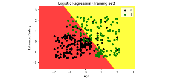
The graph shows that all points that fall in the yellow region, including the black ones, are considered 0 (Not-purchase), and all points that fall in the red area, including green ones, are considered 1 (Purchase).
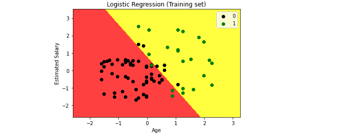
Visualizing test dataset
We will use the same method to visualize the test set result. The code for the test set will remain the same as above, except that here we will use x_test and y_test instead of x_train and y_train.
# seting x_train and y_train
x_set, y_set = X_test, y_test
x1, x2 = np.meshgrid(np.arange(start = x_set[:, 0].min() - 1, stop = x_set[:, 0].max() + 1, step  =0.01),
np.arange(start = x_set[:, 1].min() - 1, stop = x_set[:, 1].max() + 1, step = 0.01))
# Ploting
plt.contourf(x1, x2, classifier.predict(np.array([x1.ravel(), x2.ravel()]).T).reshape(x1.shape),
alpha = 0.75, cmap = ListedColormap(('red','yellow' )))
plt.xlim(x1.min(), x1.max())
plt.ylim(x2.min(), x2.max())
# for loop to iterate the data
for i, j in enumerate(np.unique(y_set)):
    plt.scatter(x_set[y_set == j, 0], x_set[y_set == j, 1],
        c = ListedColormap(('black', 'green'))(i), label = j)

# labeling the graph
plt.title('Logistic Regression (Training set)')
plt.xlabel('Age')
plt.ylabel('Estimated Salary')
plt.legend()
plt.show()
Output:
Evaluation of Logistic Regression algorithm for binary classification
Now, let’s evaluate the performance of our algorithm using a confusion matrix. A confusion matrix summarizes the actual and predicted outputs, showing correctly and incorrectly classified results. It contains TP, TN, FP, and FN values, which help us calculate the model’s accuracy, precision, recall, and f1-score.
Let’s first print outTP, TN, FP, and FN values:
# defining a function which takes acutal and pred values
def confusion_values(y_actual, y_pred):
    # initializing the values with zero value
    TP = 0
    FP = 0
    TN = 0
    FN = 0
    # iterating through the values
    for i in range(len(y_pred)):
        if y_actual[i]==y_pred[i]==1:
           TP += 1
        if y_pred[i]==1 and y_actual[i]!=y_pred[i]:
           FP += 1
        if y_actual[i]==y_pred[i]==0:
           TN += 1
        if y_pred[i]==0 and y_actual[i]!=y_pred[i]:
           FN += 1
    # printing the values
    print("True Positive: ", TP)
    print("False Positive:", FP)
    print("True Negative: ", TN)
    print("False Negative: ", FN)
# calling the function
confusion_values(y_test, y_pred)
Output:

Let us now visualize these values by building a confusion matrix. We need to import a seaborn module to plot the confusion matrix.
# importing the required modules
import seaborn as sns
from sklearn.metrics import confusion_matrix
# passing actual and predicted values
cm = confusion_matrix(y_test, y_pred, labels=classifier.classes_)
# write data values in each cell of the matrix
sns.heatmap(cm,annot=True)
plt.savefig('confusion.png')
Output:
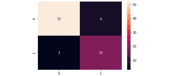
The confusion matrix shows that 52 False (Not-purchased) and 19 True classes (Purchased) were classified correctly. The model miscategorized 9 values out of 80.
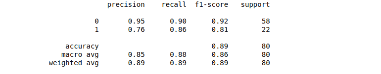
We can also print out the classification report to evaluate our model in more detail.
# importing classification report
from sklearn.metrics import classification_report
# printing the report
print(classification_report(y_test, y_pred))
Output:
Logistic regression for multiclass classification using Python
Multinomial Logistic Regression is a modified version of Logistic Regression that predicts a multinomial probability (more than two output classes) for each model input. We will use Multinomial Logistic Regression to train our model for the multiclass classification problem. In this case, we will use built-in data set for classification from the sklearn module.
Defining and exploring data sets for Multinomial logistic regression
Let’s import the classification data set from the sklearn module and other required modules we will use in our program.
# test classification dataset and counter
from collections import Counter
from sklearn.datasets import make_classification
Now, define our dataset and summarize the input and output classes.
# define dataset , number of samples 500 with 10 input features and 3 output
X, y = make_classification(n_samples=500, n_features=10, n_informative=5, n_redundant=5, n_classes=3, random_state=1)
# summarize the dataset
print(X.shape, y.shape)
print(Counter(y))
Output:

The sample size we have taken is 500 with 10 input features and 3 output classes. We can also summarize and visualize the data by pie chart as shown below:
First, we need to import the required module and then iterate through the output values and count each class to build a pie chart.
# importing numpy
import numpy as np
# creating variables
class_one = 0
class_two = 0
class_three= 0
# for loop to itreate through the output class
for i in y:
    if i ==0:
        class_one+=1
    elif i==1:
        class_two+=1
    else:
        class_three+=1
# creating numpy arry
values = np.array([class_one, class_two, class_three])
label = ["Class 0", "class 1", "class 2"]
# ploting the graph
plt.pie(values, labels = label)
plt.show()
Output:
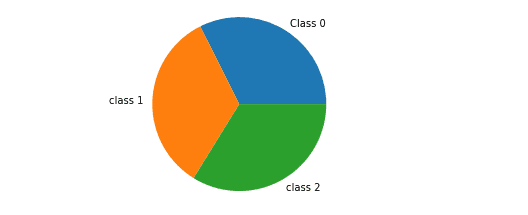
The graph shows that the training dataset is balanced (each output class has roughly the same number of representatives in the dataset).
Training the model using Multinomial Logistic Regression
Before feeding the model with data, let us divide the dataset into training and test parts to evaluate the model’s performance later.
# importing the module
from sklearn.model_selection import train_test_split
# splitting the data set into training part and testing part
X_train, X_test, y_train, y_test = train_test_split(X, y, test_size = 0.20, random_state = 1)
We can summarize the testing and training part to check how much data has been assigned to these categories.
# Summarizeing data
print("X_train : ", X_train.shape)
print("X_Test : ", X_test.shape)
print("y_train : ", y_train.shape)
print("y_test : ", y_test.shape)
Let’s now train the model by using Multinomial Logistic Regression. The Logistic Regression algorithm can be configured for Multinomial Logistic Regression by setting the multi_class argument to multinomial and the solver argument to lbfgs, or newton-cg.
# training the model
model = LogisticRegression(multi_class='multinomial', solver='newton-cg')
classifier= model.fit(X_train, y_train)
The Multinomial Logistic Regression model will fit cross-entropy loss and predict the integer value for each integer encoded class label.
Once the model training is complete, we can predict the output class by providing the testing data.
# testing the model
y_pred = classifier.predict(X_test)
# importing accuracy score
from sklearn.metrics import accuracy_score
# printing the accuracy of the model
print(accuracy_score(y_test, y_pred))
Output:

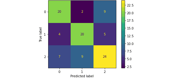
Evaluation of Multinomial Logistic Regression using a confusion matrix
You can use the confusion matrix to analyze not only the binary classification but also the multiclass classification problems. Let’s use the confusion matrix to evaluate and summarize the model’s predictions trained using Multinomial Logistic Regression on a multiclass dataset.
# importing the required modules
import matplotlib.pyplot as plt
from sklearn.metrics import confusion_matrix, ConfusionMatrixDisplay
# plot the confusion matrix in graph
cm = confusion_matrix(y_test,y_pred, labels=classifier.classes_)
# ploting with labels
disp = ConfusionMatrixDisplay(confusion_matrix=cm, display_labels=classifier.classes_)
disp.plot()
# showing the matrix
plt.show()
Output:
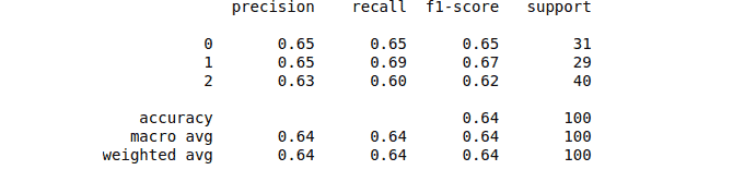
Let’s also print out the classification report for our model, which will help us know the accuracy, precision, recall, and f1-score.
# importing classification report
from sklearn.metrics import classification_report
# printing the report
print(classification_report(y_test, y_pred))
Output:
Logistic Regression using Python and AWS SageMaker Studio
Amazon SageMaker Studio provides a single, web-based visual interface where you can perform all ML development steps, improving data science team productivity by up to 10x. SageMaker Studio gives you complete access, control, and visibility into each step required to build, train, and deploy models. Let’s build our model in AWS SageMaker Studio:
# importing the libraries
import pandas as pd
# importing the dataset
dataset = pd.read_csv('LogisticRegressionDAta.csv')
# split the data into inputs and outputs
X = dataset.iloc[:, [0,1]].values
y = dataset.iloc[:, 2].values
# training and testing data
from sklearn.model_selection import train_test_split
# assign test data size 20%
X_train, X_test, y_train, y_test = train_test_split(X, y, test_size= 0.2, random_state=0)
# importing standardScaler
from sklearn.preprocessing import StandardScaler
# scalling the input data
sc_X = StandardScaler()
X_train = sc_X.fit_transform(X_train)
X_test = sc_X.fit_transform(X_test)
# importing the logistic regression from sklearn module
from sklearn.linear_model import LogisticRegression
# fitting Logistic Regression to the training set
classifier= LogisticRegression()
classifier.fit(X_train, y_train)
# testing the model
y_pred = classifier.predict(X_test)
# importing accuracy score
from sklearn.metrics import accuracy_score
# printing the accuracy of the model
print(accuracy_score(y_test, y_pred))
Output:

Summary
Logistic Regression is a Supervised learning classification algorithm used to predict the probability of a target variable. You can use it for binary and multiclass classification problems. This article demonstrated the Logistic Regression implementation for binary and multi-classification problems using Python, AWS SageMaker Studio, and Jupyter Notebook.
