Gradient Boosting for Classification and Regression
Boosting algorithms are an ensemble learning technique that allows the merging of different simple models to generate the ultimate model output. Instead of just one model on a dataset, boosting algorithm can combine models and apply them to the dataset, taking the average of the predictions made by all the models. In this process, all models are trained sequentially so that each model tries to compensate weaknesses of its predecessor. The Gradient Boosting Algorithm is one of the boosting algorithms helping to solve classification and regression problems. This article will cover the Gradient Boosting Algorithm and its implementation using Python. We will be using Amazon SageMaker Studio and Jupyter Notebooks for implementation purposes.
Table of contents
The Gradient Boosting Algorithm is also known as Gradient Tree Boosting, Stochastic Gradient Boosting, or GBM. This algorithm allows you to assemble an ultimate training model from simple prediction models, typically decision trees. Before going ahead, make sure you have a solid understanding of the Decision Tree Algorithm as Gradient Boosting Algorithm relies on it heavily. You can learn more about the Decision Tree Algorithm from the Implementing Decision Tree Using Python article.
Gradient Boosting Algorithm for a regression problem
A Gradient Boost Algorithm starts its training process from creating a single leaf from the output dataset values. This leaf is the initial guess for the output values of the dataset. During its execution, the algorithm builds new Decision Trees based on the errors’ values calculated from previous trees outputs. For example, in the case of continuous target variables, the initial guess of the Gradient Boost Algorithm will be the mean of the target (output) variable.
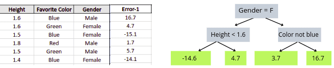
Let’s take a simple example of a regression dataset where the person’s weight will represent the output variable. Let’s also limit the Gradient Boosting Algorithm and allow the Decision Tree to have onlt 4 leaves. We’re choosing 4 leaves in this example just to have the ability to illustrate it.
So, here’s our dataset:
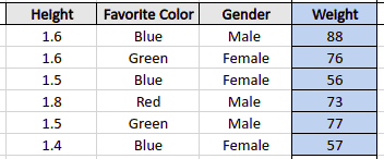
The dataset above contains three independent features (hight, favorite color, and gender) and one continuous dependent variable (weight).
We need to limit our example even more and allow the Gradient Boosting Algorithm having a limited number of Decision Trees. Again, to simplify our example, let’s agree that the algorithm will use only 2 Decision Trees for training the model and getting predictions.
The first thing that the Gradient Boosting Algorithm will do is create a leaf, and the prediction value stored in the leaf will be the mean value of the output class (weight). This will be the first prediction of the algorithm for all training data. So, if we stop the Gradient Boosting Algorithm right now, then for every row from the training dataset the algorithm will “predict” the same weight (the mean of the output class/column).
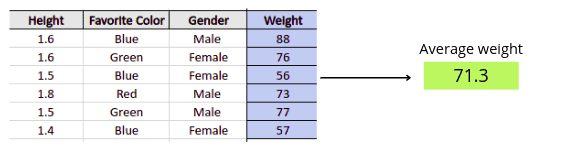
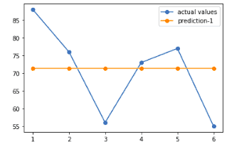
In our example, the average weight is 71.3. Let’s plot the graph of the training predictions and actual predictions at this step:
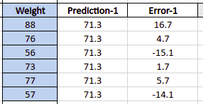
The next step of the algorithm is to build a Decision Tree based on the errors obtained from the first step. The algorithm calculates these errors as the difference between the actual weight values and the predicted weight value for every row of the training dataset.
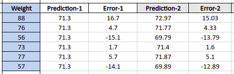
Let’s calculate these errors and store them in a new column (error-1):
The Gradient Boosting Algorithm will start building a new Decision Tree based on the Height, Favorite Color, and Gender to calculate the Error-1 column values.
Let’s say that the algorithms created the following Decision Tree and calculated the error-1 column values:

Because we have restricted the number of allowed leaves for the tree to 4, single leaf can contain more than one output. In such case, the algorithm will use the mean of the leaf values:
Now, it’s time to mention one of the important parameters that the Gradient Boosting Algorithm uses to adjust its predictions – the learning rate. Learning rate defines how “fast” the algorithm learns and adjust predicted values for the next tree. It out example, we will use 0.1 as the learning rate.
The Gradient Boosting Algorithm will use errors calculated by the Decision Tree to improve the algorithm’s prediction for the output class (it was 71.3 for all training dataset rows). The next predicted value by the Gradient Boosting Algorithm will be calculated as:
new prediction value = previous average prediction value + (learning rate) * (previous prediction error)
For example, for the first row of our sample training dataset, the algorithm will calculate the new output value (weight) as:
71.3 + 0.1 ( 16.7) = 72.97
The actual value of weight in the first row is 88, and at this step, the algorithm adjusted its prediction of the weight to the 72.97, which is a bit better than we had during the previous attempt.
Similarly, it will calculate the new predicted values and errors for each row:
Let’s visualize new model’s predictions to see how they have been improved:
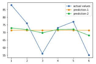
As you can see, the margin of errors between the actual and the predicted values have decreased this time compared to the first attempt of the algorithm. This is how the Gradient Boosting Algorithm “learns” from the errors made by the previous predictions while using Decision Trees.
Let’s add one more Decision Tree and train our model again to get new predictions:

The algorithm will use the same learning rate to get new better predictions as it got previously:

Let’s plot the outcomes and compare them with the previous ones:
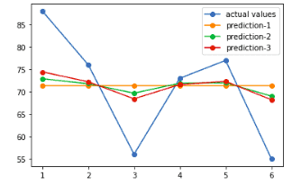
Our model at this step is trained a bit better in comparison to previous two times. Because we had specified the maximum number of trees to be 2, the red line in the above graph will be the best-fitted model. In other words, we will make predictions based on the red line in the model.
So, the mode Decision Trees you’re using, the better the outcome you should expect. The default number of decision trees in the Gradient Boosting Algorithm implementation sklearn module is 100.
The exact process repeats over and over again to get better predictions. And the entire process will stop once the algorithm reaches the maximum number of specified Decision Trees.
Gradient Boosting Algorithm for classification problems
The Gradient Boosting Algorithm can also be used to predict the categorical target variables. So now, let’s apply the Gradient Boosting Algorithm to a sample classification dataset to see how it works. But before going into the Gradient boosting for classification problems, make sure that you have a solid understanding of Logistic Regression because Gradient boosting for classification and logistic regression have many common things.
We will use the following sample data to understand how the Gradient Boosting Algorithm solves classification problems:

Our dataset contains three independent variables (like popcorn, age, and favorite season) and one target output class: whether people loved the movie or not.
We can use the Gradient Boosting Classifier to train the model on the provided data to predict the output class. The steps the Gradient Boosting Algorithm will follow in this case are similar to the regression example. The only difference here is that how the first leaf value is calculated. In the case of the classification dataset, the first leaf value is calculated as
log(odds)
As soon as 4 people from our dataset loved the movie and 2 peopled didn’t love the movie, the log(odds) value will be 0.7.
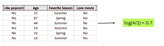
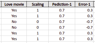
By default, the threshold value for the algorithm equals 0.5, which means any value of log(odds) above 0.5 will be considered a Yes. Because the value of log(odds) on the sample dataset is 0.7, the algorithm will consider every output as Yes. So, our first prediction for every data point will be Yes.
We can plot the above dataset and the predicted values on a graph and find the error values for each prediction:

The next step is to find errors and create a new column of the errors because the model will use these errors to improve its next predictions. Errors are calculated as the difference between the predicted and actual values.
In our case, the Yes is denoted by 1, and the No is denoted by 0.
The next steps are similar to the regression example from the above section. Depending on the number of specified Decision Trees, the algorithm will create a new tree based on the previous errors and adjust its predictions.
Implementation of Gradient Boosting Algorithm for regression problem
We already know that a regression problem is a dataset where the output class contains the continuous variables. This section will be using the diabetes dataset from the sklearn module. The dataset contains age, sex, body mass index, average blood pressure, and six blood serum measurements from diabetes patients as independent variables. The variable of interest/target is the quantitative measure of disease progression. We will use the Gradient boost regressor to train on the dataset and predict the quantitative measure of the disease.
Before going to the implementation part, make sure that you have installed the following required modules:
- sklearn
- NumPy
- Pandas
- seaborn
- plotly
You can install the required modules by running the following commands in the cell of the Jupyter notebook:
%pip install sklearn
%pip install pandas
%pip install numpy
%pip install seaborn
%pip install plotly
Once the modules are installed, we can start the implementation part then.
Importing and exploring the dataset
We can easily import the diabetes dataset from the sklearn module by importing its datasets submodule.
# importing the dataset from sklearn module
from sklearn import datasets
# loading the dataset
dataset= datasets.load_diabetes()
We will now convert our dataset to pandas DataFrame to easily explore the dataset.
# importing the pandas
import pandas as pd
# convertig the dataset into pandas dataframe
data = pd.DataFrame(dataset.data, columns=dataset.feature_names)
# printing the head
data.head(5)
Output:

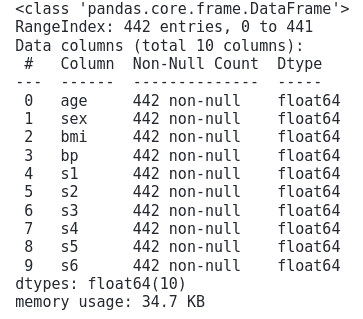
We will now apply the info() method to get more information about the dataset.
# info method
data.info()
Output:
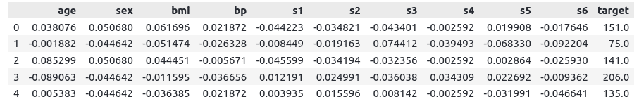
Now, let’s merge the target variable to our dataset and print out the first few rows.
# merging the target variable
data['target'] = dataset.target
# heading
data.head(5)
Output:
Splitting dataset
Before implementing the Gradient boosting regressor on our dataset, let us first split the dataset into dependent and independent variables and the testing and training dataset.
# splitting the data into inputs and outputs
Input, output = datasets.load_diabetes(return_X_y=True)
The next step is to split the data into the testing and training parts. We will assign 25% of the data to the testing and the remaining 75% to the training part.
# importing the module
from sklearn.model_selection import train_test_split
# splitting the dataset
X_train, X_test, y_train, y_test = train_test_split(Input, output, test_size=0.25)
Once the splitting is complete, we are ready to go to the implementation of the Gradient Boosting Algorithm.
Using 2 Decision Trees
As we had learned, the Gradient Boosting Algorithm creates a specified number of decision trees, and each of the decision trees helps and contributes to having the final results more accurate. In this section, we will start the training of the Gradient Boosting Algorithm by setting the number of decision trees to be 2.
The estimators represent the number of decision trees in the forest – usually, the higher the number of trees, the better result you might get. But let’s start training the model from two estimators first.
# Importing the Gradient Boosting Regressor
from sklearn.ensemble import GradientBoostingRegressor
# training
GB_regressor=GradientBoostingRegressor(n_estimators=2)
GB_regressor.fit(X_train,y_train)
The next step is to test the model by providing the testing dataset.
# predicting
GB_predict=GB_regressor.predict(X_test)
Let’s plot the actual values and values predicted by our model:
# creating x_axis for simplicity
x_axis = [i for i in range(len(y_test))]
# importing the module
import matplotlib.pyplot as plt
# fitting the size of the plot
plt.figure(figsize=(15, 8))
# plotting the graphs
plt.plot(x_axis,GB_predict, label="Predicted values")
plt.plot(x_axis,y_test, label="actual values")
plt.legend()
plt.show()
Output:

Our predictions are not as good as actual values. This happened because we have used only two Decision Trees.
We can also use various evaluation matrices to see the performance of our model. But here, we will only consider the Mean Absolute Error (MAE) and R2 score to evaluate the model:
# Importing mean_absolute_error from sklearn module
from sklearn.metrics import mean_absolute_error, r2_score
# Evaluating the model
print('MAE is :', mean_absolute_error(y_test, GB_predict))
print('R score is :', r2_score(y_test, GB_predict))
Output:

The lower the value of MAE will be, the better the algorithm performs. At the same time, the value of the R2-score is between 0 and 1, and the closer the value to 1, the better the algorithm has performed.
Using 10 Decision Trees
Now let’s increase the number of estimators and see how it affects the model’s predictions. We will not change/or alter any other parameters. They were already set to their default values.
# training on 10 estimator
GB_regressor=GradientBoostingRegressor(n_estimators=10)
GB_regressor.fit(X_train,y_train)
# predicting
GB_predict=GB_regressor.predict(X_test)
Let’s visualize the model predictions:
# fitting the size of the plot
plt.figure(figsize=(15, 8))
# plotting the graphs
plt.plot(x_axis,GB_predict, label="Predicted values")
plt.plot(x_axis,y_test, label="actual values")
plt.legend()
plt.show()
Output:
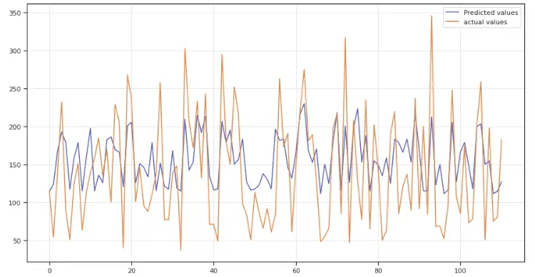
As you can see, the predicted values (blue line) much better fits the actual data, but still not good enough.
We can also use the same evaluation matrices to evaluate the model and compare the model’s performance with the previous one using numerical values.
# Evaluating the model
print('MAE is :', mean_absolute_error(y_test, GB_predict))
print('R score is :', r2_score(y_test, GB_predict))
Output:

At this time we’ve got lower value for MAE and a more significant value for R-score.
It is always challenging to set up an optimum number of Decision Trees for the algorithm. In such a case, GridSearchCV can help you to find the optimum number of Decision Trees for your model.
Using GridSearchCV to find the best parameters
GridSearchCV class allows you to search through the best parameters’ values from provided range of parameters. Basically, it calculates model’s performance for every single combination of provided parameters and outputs the best parametes’ combination.
Let’s use the GridSearchCV helper class to find our model’s optimum number of estimators:
# importing required module
from sklearn.model_selection import GridSearchCV
# initializing the model
model=GradientBoostingRegressor()
# defining the estimators to be in range of 100
params={'n_estimators':range(1,100)}
# applying GridSearchCV
grid=GridSearchCV(estimator=model,cv=2,param_grid=params,scoring='neg_mean_squared_error')
# training the model
grid.fit(X_train,y_train)
# printing the best estimator
print("The best estimator returned by GridSearch CV is:", grid.best_estimator_)
Output:

So, the optimum number of estimators returned by the GridSearchCV is 26. Let’s check out how our model would perform using this number of estimators.
# training
GB_regressor=GradientBoostingRegressor(n_estimators=26)
GB_regressor.fit(X_train,y_train)
# predicting
GB_predict=GB_regressor.predict(X_test)
Once the training and prediction are complete, we can visualize results again:
# fitting the size of the plot
plt.figure(figsize=(15, 8))
# plotting the graphs
plt.plot(x_axis,GB_predict, label="Predicted values")
plt.plot(x_axis,y_test, label="actual values")
plt.legend()
plt.show()
Output:
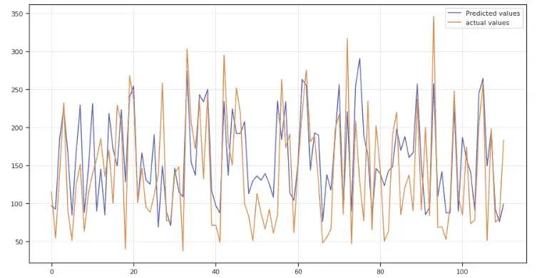
This time, the best-fitted line is close to the actual value compared to previous attempts. Let’s find the MAE and R2-score of the model:
# Evaluating the model
print('MAE is :', mean_absolute_error(y_test, GB_predict))
print('R score is :', r2_score(y_test, GB_predict))
Output:

As you can see, we’ve got much better accuracy than in previous attempts.
Implementation of Gradient Boosting Algorithm for classification problem
Now, let’s apply the Gradient Boosting Algorithm to solve a classification problem (output classes contain categorical values). We’ll use a famous sklearn built-in Iris dataset containing information about different flower species.
The Iris dataset contains input variables such as sepal width, petal width, sepal length, and petal length or Iris flowers. The output class represented by three different types of flowers based on their petal and sepal sizes. This section will apply the Gradient Boosting Algorithm to predict the type of flower based on the sepal and petal size.
Importing and exploring the dataset
The datasets submodule allows you to get the Iris dataset. Let’s import the dataset, convert it to pandas DataFrame, and print a few rows:
# importing the dataset
dataset = datasets.load_iris()
# convertig the dataset into pandas dataframe
data = pd.DataFrame(dataset.data, columns=dataset.feature_names)
# printing the independent column
data.head()
Output:

The output contains all independent variables. Now, let’s add the target (output) variable to the dataset as well.
# merging the target variable
data['target'] = dataset.target
# printing
data.head(5)
Output:

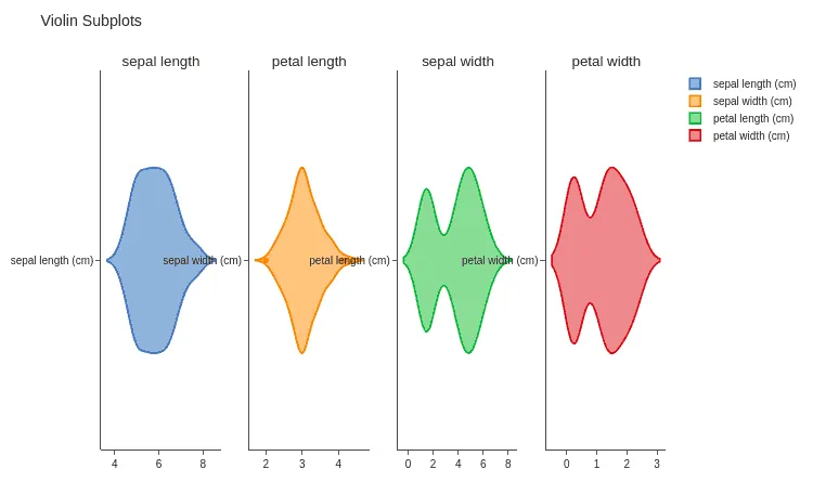
To see the distribution of each of the independent variables, we can use the violin plot:
#importing the required modules
from plotly.subplots import make_subplots
import plotly.graph_objects as go
# creating subplot
fig = make_subplots(rows=1, cols=4,subplot_titles=("sepal length","petal length","sepal width","petal width"))
# creating volin plot for sepal length
fig.append_trace(go.Violin(x=data['sepal length (cm)'],name='sepal length (cm)'), row=1, col=1)
# creating volin plot for the sepal width
fig.append_trace(go.Violin(x=data['sepal width (cm)'],name='sepal width (cm)'), row=1, col=2)
# creating  volin plot for the petal length
fig.append_trace(go.Violin(x=data['petal length (cm)'],name='petal length (cm)'), row=1, col=3)
# creating volin plot for the petal width
fig.append_trace(go.Violin(x=data['petal width (cm)'],name='petal width (cm)'), row=1, col=4)
# showing the graph
fig.update_layout(height=600, width=900, title_text="Violin Subplots", template="simple_white")
fig.show()
Output:
Splitting the dataset
Before applying the Gradient Boosting Classifier, we need to split our dataset into independent and dependent variables along with the testing and training part:
# splitting the data into inputs and outputs
Input, output = datasets.load_iris(return_X_y=True)
Now, we will split the dataset into the testing and training parts. We will specify 30% for the testing and the remaining 70% for the training.
# importing the module
from sklearn.model_selection import train_test_split
# splitting the dataset
X_train, X_test, y_train, y_test = train_test_split(Input, output, test_size=0.30)
Now, our dataset is ready to train the model and test it.
Applying Gradient Boosting Classifier
Let’s apply the Gradient Boosting Classifier on the dataset to train the model and then use trained model to predict the output category of flowers.
# importing the required module
from sklearn.ensemble import GradientBoostingClassifier
# training with default values
GB_classifier=GradientBoostingClassifier()
GB_classifier.fit(X_train,y_train)
Once the training is complete, we can test our model by providing the testing data.
# predicting
GB_predict=GB_classifier.predict(X_test)
Now let us evaluate the model by finding the accuracy.
# importing the module
from sklearn.metrics import accuracy_score
# printing
print("The accuracy is: ", accuracy_score(y_test, GB_predict))
Output:

The output shows that our model has accurately classified 95% of the testing data, which is a good result.
Evaluating Gradient Boosting Classifier using confusion matrix
A confusion matrix is a table that is often used to describe the performance of a classification model (or “classifier”) on a set of test data. Learn more about the confusion matrix and its usage for evaluating the classifier model from the evaluation of the KNN algorithm.
Let’s use the confusion matrix to visualize the prediction and the actual values:
# importing the modules
import seaborn as sns
from sklearn.metrics import confusion_matrix
import matplotlib.pyplot as plt
# providing actual and predicted values
cm = confusion_matrix(y_test, GB_predict)
# If True, write the data value in each cell
sns.heatmap(cm,annot=True)
# saving confusion matrix in png form
plt.savefig('confusion_Matrix.png')
Output:
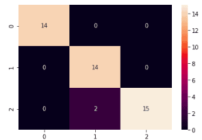
The output shows that the model incorrectly predicted only two values.
Let’s print the classification report, which shows us the model’s accuracy, precision, and R2-score:
# importint the module
from sklearn.metrics import classification_report
# printing the report
print(classification_report(y_test, GB_predict))
Output:

We hope that you’re able to interpret model performance results by yourself.
Summary
Gradient Boosting Algorithm is a Machine Learning algorithm that tries to create a more accurate model by combining previous models, minimizing the overall prediction error. The key idea is to use the previous model’s outcomes to reduce the error of the next applied model. This article covered the Gradient Boosting Algorithm in detail by reviewing its implementation steps for solving regression and classification problems.
