Implementation of Hierarchical Clustering using Python

Unsupervised Machine Learning uses Machine Learning algorithms to analyze and cluster unlabeled datasets. The most efficient algorithms of Unsupervised Learning are clustering and association rules. Hierarchical clustering is one of the clustering algorithms used to find a relation and hidden pattern from the unlabeled dataset. This article will cover Hierarchical clustering in detail by demonstrating the algorithm implementation, the number of cluster estimations using the Elbow method, and the formation of dendrograms using Python. We will use Jupyter Notebook and AWS SageMaker Studio for implementation and visualization purposes.

What is Hierarchical Clustering?

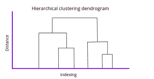
Hierarchical clustering is another Unsupervised Machine Learning algorithm used to group the unlabeled datasets into a cluster. It develops the hierarchy of clusters in the form of a tree-shaped structure known as a dendrogram. A dendrogram is a tree diagram showing hierarchical relationships between different datasets.

Sometimes the results of K-means clustering and hierarchical clustering may look similar, but they both differ depending on how they work.

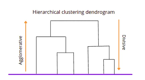
Hierarchical clustering uses two different approaches to create clusters:

• Agglomerative is a bottom-up approach in which the algorithm starts with taking all data points as single clusters and merging them until one cluster is left.
• Divisive is the reverse to the agglomerative algorithm that uses a top-bottom approach (it takes all data points of a single cluster and divides them until every data point becomes a new cluster).

One of the most significant advantages of Hierarchical over K-mean clustering is the algorithm doesn’t need to know the predefined number of clusters. We can assign the number of clusters depending on the dendrogram structure.

How Hierarchical clustering algorithm works?

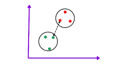
Let’s focus on the Agglomerative method to describe how the Hierarchical clustering algorithm works. This method starts joining data points of the dataset that are the closest to each other and repeats until it merges all of the data points into a single cluster containing the entire dataset.

For example, let’s take six data points as our dataset and look at the Agglomerative Hierarchical clustering algorithm steps.

The very first step of the algorithm is to take every data point as a separate cluster. If there are N data points, the number of clusters will be N.

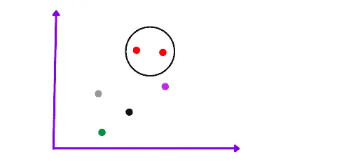
The next step of this algorithm is to take the two closest data points or clusters and merge them to form a bigger cluster. The total number of clusters becomes N-1.

Subsequent algorithm iterations will continue merging the nearest two clusters until only one cluster is left.

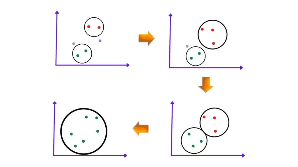
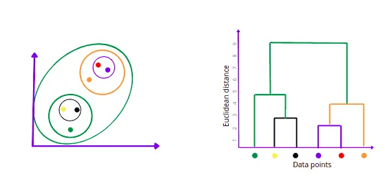
Once the algorithm combines all the data points into a single cluster, it can build the dendrogram describing the clusters’ hierarchy.

Measuring distance bewteen two clusters

The distance between clusters or data points is crucial for Hierarchical clustering. Several Linkage methods can calculate this distance:

Single linkage is the shortest distance between the closest points of the clusters calculated by any distance finding method (the most popular is the Euclidean distance).

Complete linkage is the longest distance between the two points of two different clusters. This linkage method allows you to create tighter clusters than a single linkage approach.

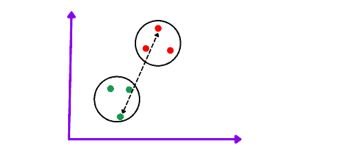
Centroid Linkage is the distance between the centroid of two clusters.

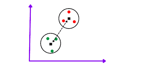
Depending on the Python modules, there may be other ways to measure the distance between clusters. Please, refer to module documentation to get a better understanding of what’s exactly measured.

Dendrogram in Hierarchical clustering

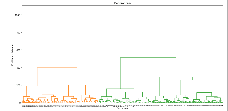
The dendrogram is a tree-like structure that stores each step of the Hierarchical algorithm execution process. In the Dendrogram plot, the x-axis shows all data points, and the y-axis shows the distance between them. The below dendrogram describes the formation of clusters.

Once we have the dendrogram for the clusters, we can set a threshold (a red horizontal dashed line) to visually see the number of output classes from the dataset after algorithm execution.

Threshold is minimum distance required between the nearest clusters to treat them as a separate clusters. This is knowledge domain variable which you need to define yourself. If you don’t have enough information about your business domain, you can use the following methods to define the number of clusters in the dataset (take a look at the “7 methods for selecting the optimal number of clusters” article to find the implementation code).

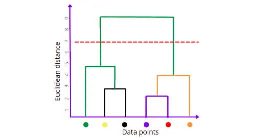
For example, for the threshold value of 7, the number of clusters will be 2. For the threshold value equal to 3, we’ll get 4 clusters, etc.

Hierarchical clustering algorithm implementation

Let’s implement the Hierarchical clustering algorithm for grouping mall’s customers (you can get the dataset here) using Python and Jupyter Notebook.

In this example, we’ll be interested in segmenting customers into groups based on their sales, needs, etc. Business owners may use this segmentation to work with every customer segment individually and improve relationships between the company and customers or increase revenue from the specific customer category.

To split customers into categories, we need the following Python modules:

• skearn
• matplotlib
• pandas
• numpy
• seaborn
• plotly
• yellowbrick

You can install these modules by running the following commands in the cell of the Jupyter Notebook:

%pip install sklearn
%pip install matplotlib
%pip install pandas
%pip install numpy
%pip install seaborn
%pip install plotly
%pip install yellowbrick
%pip install chart_studio

In this section, we will be using Mall customer segmentation data. You can download the dataset from this link.

Exploring and preparing dataset

Let’s import the dataset using pandas module.

# importing the module
import pandas as pd
# importing the dataset
dataset = pd.read_csv('Hierarchical_clustering_data.csv')
# dataset 
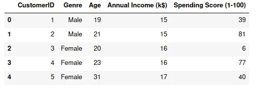
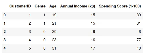
dataset.head()

Output:

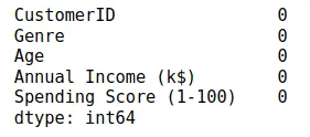
The next important step is to check if our dataset contains any null values. The DataFrame class of the Pandas module provides the isnull() method which returns the count of null values, if any.

# checking for null values
dataset.isnull().sum()

Output:

Let’s visualize each of these variables (Age, Annual Income, and Spending Score) using distplot to see the distribution of the values for each column.

# importing the required modules
import matplotlib.pyplot as plt
import seaborn as sns
# graph size
plt.figure(1 , figsize = (15 , 6))
graph = 0 
# for loop
for x in ['Age' , 'Annual Income (k$)' , 'Spending Score (1-100)']:
    graph += 1
    
    # ploting graph
    plt.subplot(1 , 3 , graph)
    plt.subplots_adjust(hspace = 0.5 , wspace = 0.5)
    sns.distplot(dataset[x] , bins = 15)
    plt.title('Distplot of {}'.format(x))
# showing the graph
plt.show()

Output:

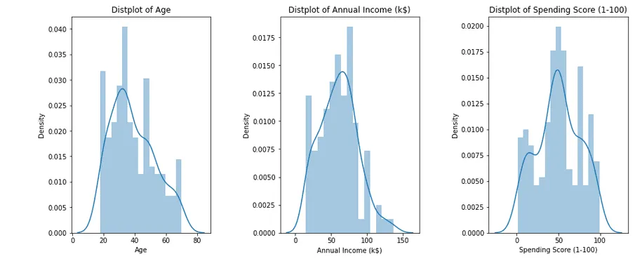
The output shows that all values in our columns fit an almost normal distribution.

Our dataset contains one column (Genre) with string values, so we need to encode these values to numeric values before applying the algorithm.

# importing preprocessing 
from sklearn import preprocessing 
# lable encoders
label_encoder = preprocessing.LabelEncoder() 
# converting gender to numeric values
dataset['Genre'] = label_encoder.fit_transform(dataset['Genre'])
# head
dataset.head()

Output:

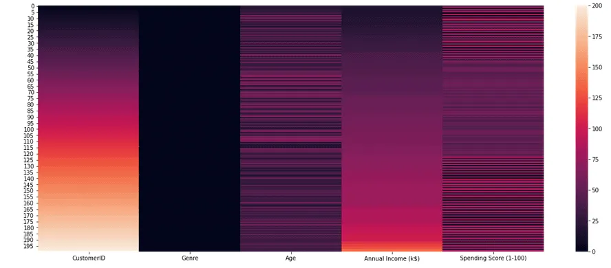
Another way to understand the intensity of data clusters is using a heat map. A heat map is a data visualization technique that shows the magnitude of a phenomenon as color in two dimensions. The color variation may be by hue or intensity, giving obvious visual cues to the reader about how the phenomenon is clustered or varies over space.

# graph size
plt.figure(1, figsize = (20 ,8))
# creating heatmap
sns.heatmap(dataset)
# showing graph
plt.show()

Output:

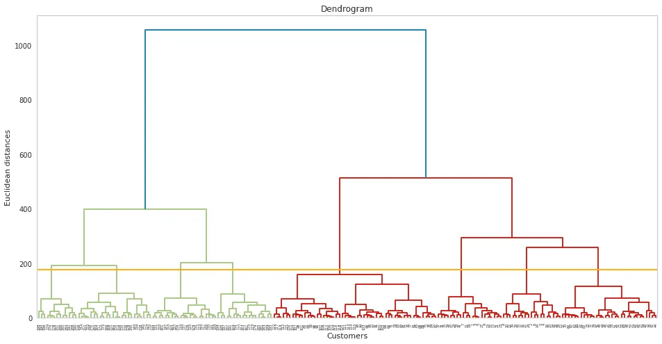
Visvualizing Dendrogram

Now we can find the optimal number of clusters and the approximate threshold value.

Let’s use scipy module, which can automatically build the dendrogram for the dataset.

# importing the required module
import scipy.cluster.hierarchy as sch
# graph size
plt.figure(1, figsize = (16 ,8))
# creating the dendrogram
dendrogram = sch.dendrogram(sch.linkage(dataset, method  = "ward"))
# ploting graphabs
plt.title('Dendrogram')
plt.xlabel('Customers')
plt.ylabel('Euclidean distances')
plt.show()

Output:

Using Elbow method for estimating number of clusters

The Elbow method allows you to estimate the meaningful amount of clusters we can get out of the dataset by iteratively applying a clustering algorithm to the dataset providing the different amount of clusters, and measuring the Sum of Squared Errors or inertia’s value decrease. Let’s use the Elbow method to our dataset to get the number of clusters estimation:

# Import ElbowVisualizer
from sklearn.cluster import AgglomerativeClustering
from yellowbrick.cluster import KElbowVisualizer
model = AgglomerativeClustering()
# k is range of number of clusters.
visualizer = KElbowVisualizer(model, k=(2,30), timings=False)
# Fit data to visualizer
visualizer.fit(dataset)
# Finalize and render figure
visualizer.show()

Output:

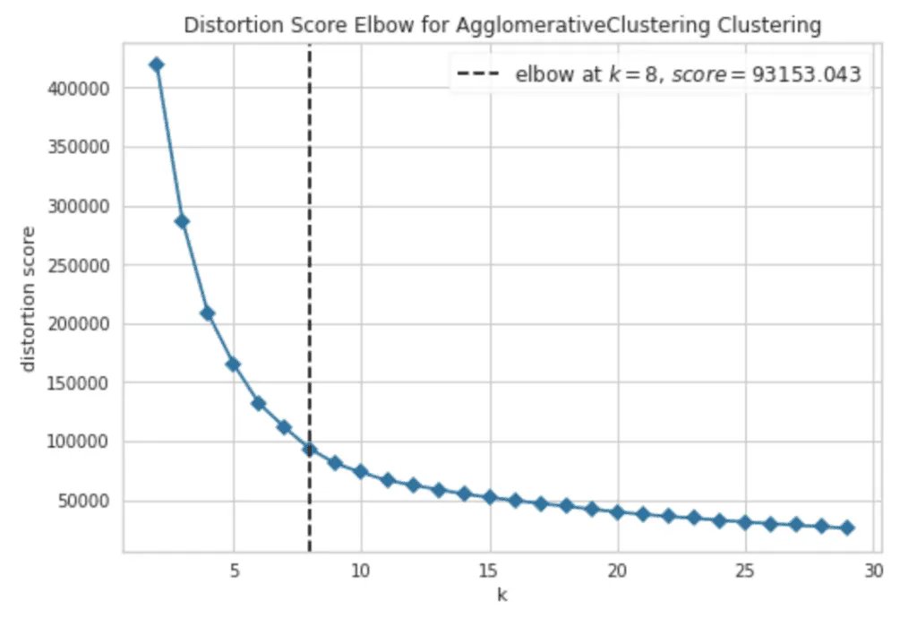
The output plot shows that the best number of clusters we can get out of our dataset is 8.

Based on this information, we can assume that the threshold value for this dataset might be approximately 175.

import scipy.cluster.hierarchy as sch
# size of image
plt.figure(1, figsize = (16 ,8))  
plt.grid(b=None)
# creating the dendrogram 
dend = sch.dendrogram(sch.linkage(dataset, method='ward'))
# theroshold
plt.axhline(y=175, color='orange')
# ploting graphabs
plt.title('Dendrogram')
plt.xlabel('Customers')
plt.ylabel('Euclidean distances')
plt.show()

Output:

Implementing Agglomerative Hierarchical clustering

Now, let’s take the clusters (8) and visualize them. We have three main variables (Age, Spending score, and Annual income), which we can put on a 3D plot to see clustered data distribution.

import plotly as plt
import plotly.graph_objects as go
# calling the agglomerative algorithm
model = AgglomerativeClustering(n_clusters = 8, affinity = 'euclidean', linkage ='average')
# training the model on dataset
y_model = model.fit_predict(dataset)
# creating pandas dataframe
dataset['cluster'] = pd.DataFrame(y_model)
# creating scattered graph
trace1 = go.Scatter3d(
    
    # storing the variables in x, y, and z axis
    x= dataset['Age'],
    y= dataset['Spending Score (1-100)'],
    z= dataset['Annual Income (k$)'],
    mode='markers',
     marker=dict(
        color = dataset['cluster'], 
        size= 3,
        line=dict(
            color= dataset['cluster'],
            width= 12
        ),
        opacity=0.9
     )
)
# ploting graph 
data = [trace1]
layout = go.Layout(
    title= 'Clusters using Agglomerative Clustering',
    scene = dict(
            xaxis = dict(title  = 'Age'),
            yaxis = dict(title  = 'Spending Score'),
            zaxis = dict(title  = 'Annual Income')
        ),
    width=1024, height=512
)
fig = go.Figure(data=data, layout=layout)
plt.offline.iplot(fig)

Output:

Summary

Hierarchical clustering is an Unsupervised Learning algorithm that groups similar objects from the dataset into clusters. This article covered Hierarchical clustering in detail by covering the algorithm implementation, the number of cluster estimations using the Elbow method, and the formation of dendrograms using Python.