Implementation of XGBoost algorithm using Python

Boosting algorithms are an ensemble learning technique that allows the merging of different simple models to generate the ultimate model output. Instead of using just one model on a dataset, boosting algorithm can combine models and apply them to the dataset, taking the average of the predictions made by all the models. XGBoost (eXtreme Gradient Boosting) is a widespread and efficient open-source implementation of the gradient boosted trees algorithm. Gradient boosting is a supervised learning algorithm that attempts to accurately predict a target variable by combining the estimates of a set of simpler, weaker models. This article will cover the XGBoost algorithm implementation and apply it to solving classification and regression problems. We will be using AWS SageMaker Studio and Jupyter notebooks for implementation and visualization purposes.

Understanding the working principle of the XGBoost algorithm will be easy if you already understand how the Gradient boosting algorithm is working.

Best Machine Learning Books for Beginners and Experts

As Machine Learning becomes more and more widespread, both beginners and experts need to stay up to date on the latest advancements. For beginners, check out the best Machine Learning books that can help to get a solid understanding of the basics. For experts, reading these books can help to keep pace with the ever-changing landscape. In either case, a few key reasons for checking out these books can be beneficial.

First, they provide a comprehensive overview of the subject matter, mainly about Machine Learning algorithms. Second, they offer insights from leading experts in the field. And third, they offer concrete advice on how to apply Machine Learning concepts in real-world scenarios. As Machine Learning continues to evolve, there’s no doubt that these books will continue to be essential resources for anyone with prior knowledge looking to stay ahead of the curve.

Explanation of XGBoost algorithm

XGBoost (eXtreme Gradient Boosting) is a widespread and efficient open-source implementation of the gradient boosted trees algorithm. The following are the main features of the XGBoost algorithm:

• Regularized boosting: Regularization techniques are used to reduce overfitting. In Machine Learning, overfitting refers to when the trained model fits the training data too well. It happens when a model learns the detail and noise in the training data to the extent that it negatively impacts the model’s performance on new data.
• Handle missing values automatically: When using the XGBoost algorithm on a dataset, we don’t need to care about the missing values because the algorithm automatically handles them.
• Parallel processing: XGBoost doesn’t run multiple trees in parallel; instead, it does the parallelization within a single tree by using openMP to create branches independently.
• Cross-validation at each iteration: Cross-Validation is a statistical method of evaluating and comparing learning algorithms by dividing data into two segments: one used to learn or train a model and the other used to validate the model. XGBoost internally has parameters for cross-validation.
• Tree pruning: Pruning reduces the size of decision trees by removing parts of the tree that does not provide value to classification.

The XGBoost algorithm takes many parameters, including booster, max-depth, ETA, gamma, min-child-weight, subsample, and many more. In this article, we will only discuss the first three as they play a crucial role in the XGBoost algorithm:

• booster: defines which booster to use. By default, the booster is gbtree, but we can select gblinear or dart depending on the dataset.
• eta: ETA is the learning rate of the model. Its value can be from 0 to 1, and by default, the value is 0.3.
• max-depth – is the maximum depth of a tree. Increasing this value will make the model more complex and more likely to overfit. By default, the value is 6.

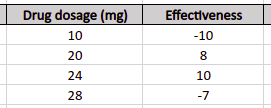
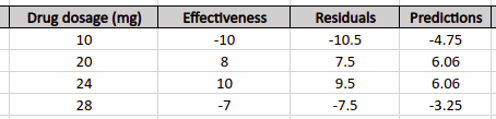
XGBoost algorithm is built to handle large and complex datasets, but let’s take a simple dataset to describe how this algorithm works. Let’s imagine that the sample dataset contains four different drugs dosage and their effect on the patient. The negative values show that the drug was not helpful, while the positive values show the opposite result.

To simplify the explanation, we will restrict the number of XGBoost trees to 1 and the depth of the tree to 2. That means we will train the XGboost training and predictions on only one tree with a depth of 2.

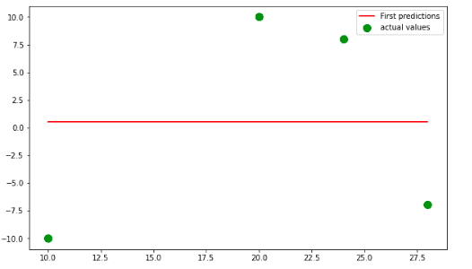
The first step that XGBoost algorithms do is making an initial prediction of the output values. You can set up output values to any value, but by default, they are equal to 0.5. The horizontal line in the graph shows the first predictions of the XGboost, while the dots show the actual values.

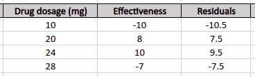
Similar to the Gradient Boosting algorithm, the next step is to calculate the residuals, the difference between the first predictions and the actual values.

Residual = actual value – Predicted value

Let’s add the Residuals to our excel sheet:

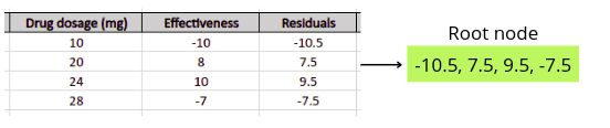
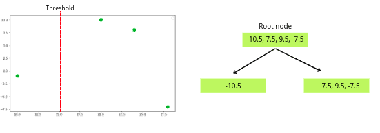
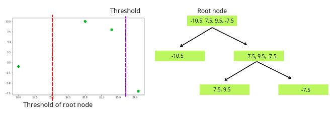
Next, the XGboost algorithm will start building the decision tree. The root node of the decision tree will contain all residuals.

After that, the algorithm will now calculate the similarity score of the node:

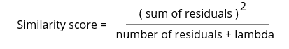
In this equation, the lambda is the regularization parameter, so let’s say its value is 1. Then the similarity score of the root node is:

Similarity score = (-10.5 + 7.5 + 9.5 – 7.5)^2 / (4+ 1)

Similarity score = 0.2

As soon as we have the root node with a similarity score, we can build different decision trees using the same root node and select the decision tree, which will be more efficient.

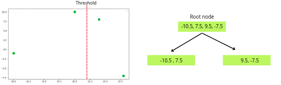
The question is, how the decision trees are going to be created? The algorithm will create different decision trees based on different threshold values. The first threshold value will be the mean of the two last samples.

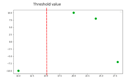
Now one decision tree will be created based on the above threshold value, as shown below.

The next step is to find the similarity score of both leaf nodes.

Similarity score of left leaf = (-10.5) ^ 2 / (1 + 1)

Simlarity score of left leaf = 55.125

Similarity score of right leaf = ( 7.5 + 9.5 -7.5 ) ^ 2 / ( 3 + 1)

Similiarity score of right leaf = 22.562

Now, it is time to find out how much the tree was successful in clustering the residuals compared to the root node. We do this by calculating the Gain of the splitting residuals into two groups.

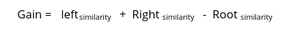
As we’ve already calculated similarity values for each node, the gain value of the decision tree will be:

Gain = 55.125 + 22.562 – 0.2

Gain = 77.48

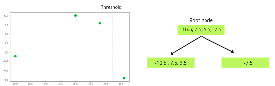
Now, we will change the threshold value to create another decision tree. The next threshold value will be the mean of the following two training data rows.

The same steps will repeat, and the algorithm will calculate the similarity scores of each of the nodes and then calculate the Gain value of the decision tree.

The similarity score of the left leaf = 3

The similarity score of the right leaf = 1.33

Gain = 4.13

Once we calculate the Gain of the tree, then again, we will change the threshold value gain to create one more decision tree.

The following steps are similar to the previous ones. We will again calculate the similarity scores of each node and then find out the gain value of the decision tree.

The similarity score of the left leaf = 10.56

The similarity score of the right leaf = 28.12

Gain = 37.925

Now we have created different decision trees based on various threshold values. The next step is to take the decision tree that is more efficient for further processing. The efficiency of the decision tree depends on the Gain value. The more the gain value is, the better the decision tree has contributed to making clusters of the training dataset. So in our case:

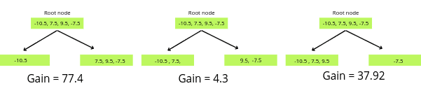
The first decision tree has created better clusters than the others, so that we will take it for further processing.

We can’t split the left node any further because it contains only one value. But we can split the right node into other nodes.

Again we will select a threshold value for the training dataset and split the dataset.

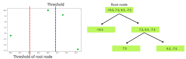
We will again find the similarity score of newly created nodes and the gain value of the decision tree.

The similarity score of the left leaf = 28.12

The similarity score of the right leaf = 1.33

Gain = 6.89

The next step is to change the threshold again and create a new decision tree.

Again we will calculate the similarity score of the nodes and the Gain value of the newly created tree.

The similarity of the left leaf = 95.33

The similarity of the right leaf = 28.12

Gain = 100.89

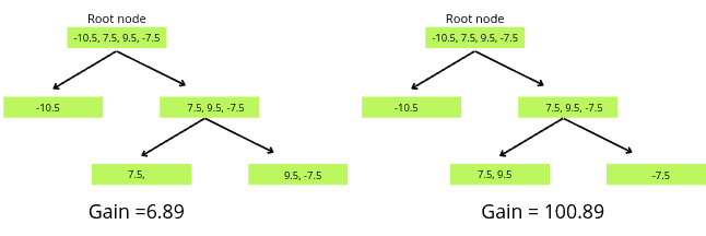
As the gain value of the second decision tree is more significant, we will consider it for training and predicting.

Note that there will be no further splitting of the leaf nodes, as we have limited the depth of tree 2.

So, the final tree that we will use for the training and predictions is:

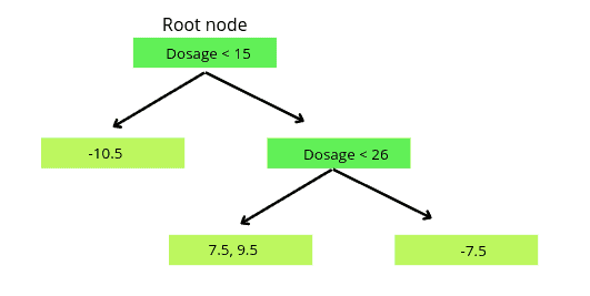
Now, based on this tree, we will predict the output values for the leaves. The output for the leave is calculated using the following formula:

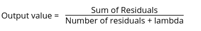
So, the output values in each of the leaves will be:

The output of the first leaf = ( -10.5 ) / ( 1+ 1) = -5.25

The output of the second leaf = (7.5 + 9.5 ) / ( 2 + 1 ) = 5.66

The output of the third leaf = ( -7.5 ) / ( 1 + 1 ) = -3.75

The predictions of the XGBoost model will be:

First predictions + ( learning rate ) * ( Decision tree’s predictions).

For this example, we will take the learning rate equal to 1. So we will have the following predicted values:

So, the best-fitted line of our model trained on a max-depth of 2 is the blue line:

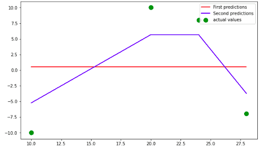
Because we have restricted the model to having only one tree, the above blue line will be the best-fitted line of our model on the given dataset. Otherwise, the model will again find the residuals based on the new predictions and then create decision trees for further predictions until the max number of decision trees is reached.

Implementation of XGBoost for a regression problem

Let’s implement the XGBoost algorithm using Python to solve a regression problem. We will use a dataset containing the prices of houses in Dushanbe city. The cost of the home depends on the area, location, number of rooms, and number of floors. You can download the dataset from this link.

Before going to the implementation part, make sure that you have installed the following Python modules:

• xgboost
• sklearn
• pandas
• numpy
• plotly
• matplotlib
• seaborn

You can install them using the pip command by running the following commands in the cell of the Jupyter notebook.

%pip install xgboost
pip install sklearn
pip install pandas
pip install numpy
pip install plotly
pip install matplotlib
pip install seaborn

Once the installation of the modules is complete, we can go to the implementation part.

Importing and exploring the dataset

We will use the Pandas module to open the dataset and explore it.

# importing the pandas module
import pandas as pd
# importing the dataset
dataset = pd.read_csv("Dushanbe_house.csv")

Let’s print a few rows of the dataset:

# printing few rows
dataset.head()

Output:

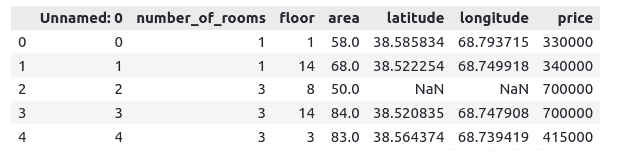
Our dataset has some null values. The XGBoost algorithm will automatically handle them.

We can plot the house’s location vs. the price to see their correlation.

# importing the required module
import plotly.express as px
# creating 3-d graph
fig = px.scatter_3d(
    x=dataset['price'], y=dataset['latitude'], z=dataset['longitude'], color=dataset['price'],
    title="3-graph"
)
fig.show()

Output:

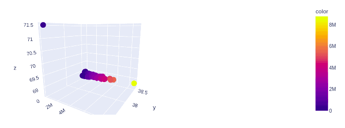
We can observe that as the location of the house changes, the price also changes. We can also infer that most houses are located in one place except for two homes.

We can also check the distribution of the prices by plotting a bar chart. We will select 200 random prices from the dataset and plot them using a bar chart.

# converting the prices to list
y = list(dataset['price'])
# importing random
import random
# creating sample of 100 random prices
y_axis = random.sample(y, 200)
# creating bar chart
fig = px.bar( x=[i for i in range(len(y_axis))], y=y_axis)
fig.show()

Output:

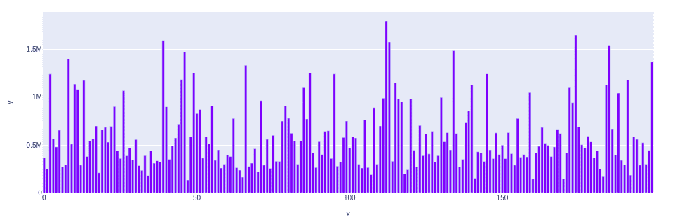
So, we can infer that the prices are randomly distributed based on the above bar plot.

Splitting dataset

We will now split the dataset into input variables and output variables.

# taking the columns from the dataset
columns = dataset.columns
# storing the input and output variables
X = dataset[columns[0:-1]]
y = dataset[columns[-1]]

The next step is to divide the dataset into testing and training parts so that we can train and then evaluate the model. We will use the sklearn module to split the dataset.

# importing the module
from sklearn.model_selection import train_test_split
# splitting the dataset
X_train, X_test, y_train, y_test = train_test_split(X, y, test_size = 0.25, random_state = 0)

We have assigned 25% of the data to the testing and 75% to the training parts.

XGBoost with default parameters

Let’s train our model using the default parameters:

# printing the default parameters of XGBoostmodel.
xgb.XGBRegressor().get_params()

Output:

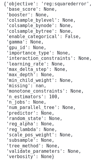
Let’s train our model without changing these parameters.

# we initiate the regression model and train it with our train data
xg_reg = xgb.XGBRegressor()
# training the model
xg_reg.fit(X_train,y_train)

Once the training is complete, we can use the testing data to predict the outcomes.

# predicting the outputs
xgb_preds = xg_reg.predict(X_test)

It is now time to see how well our model is predicting. First, let us plot a graph of the predicted and actual values.

# importing the module
import matplotlib.pyplot as plt
# fitting the size of the plot
plt.figure(figsize=(20, 8))
# plotting the graphs
plt.plot([i for i in range(len(y_test))],y_test, label="actual values")
plt.plot([i for i in range(len(y_test))],xgb_preds, label="Predicted values")
# showing the plotting
plt.legend()
plt.show()

Output:

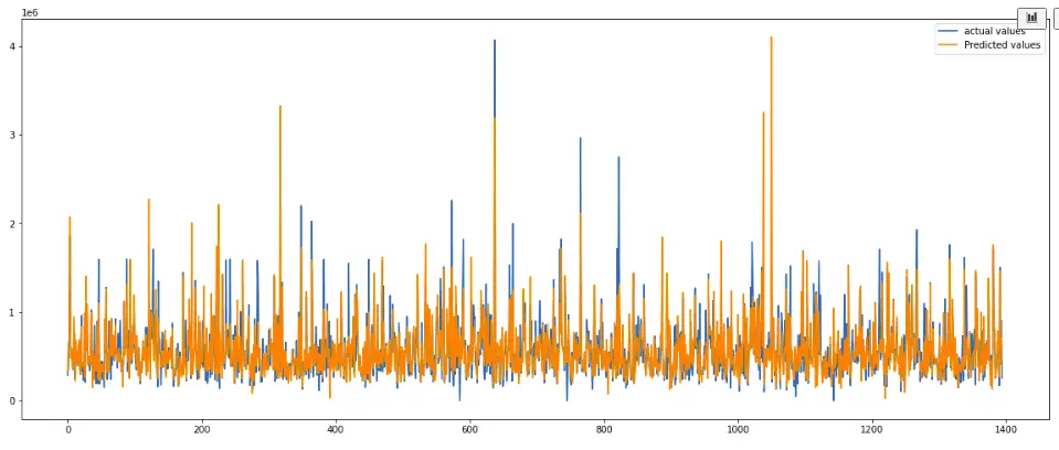
The predictions seem to be pretty good. Let’s calculate the R²-score of the predictions as well. The R²-score is usually between 0 and 1. The more the value is closer to 1, the better the model makes predictions.

# Importing the required module
from sklearn.metrics import r2_score
# Evaluating the model
print('R score is :', r2_score(y_test, xgb_preds))

Output:

The R²-score shows that the predictions are reasonable.

GridSearchCV to find the optimum parameters

The GridSearchCV helper class allows us to find the optimum parameters from a given range. Let’s use the GridSearchCV to find the optimum parameters for the XGBoost algorithm. We will apply GridSearcCV on only three-parameter. You can apply the GridSearchCV on all other parameters, but it will take a lot of time.

To keep track of time, we will create a function that will return the total time taken by GridSeachCV to find the optimum parameters’ values.

# function to print the total time
def timer(start_time=None):
    # starting the time
    if not start_time:
        start_time = datetime.now()
        return start_time
    # ending the time
    elif start_time:
        thour, temp_sec = divmod((datetime.now() - start_time).total_seconds(), 3600)
        tmin, tsec = divmod(temp_sec, 60)
        # printing the total time
        print('\n Time taken: %i hours %i minutes and %s seconds.' % (thour, tmin, round(tsec, 2)))

The above function will print the total time taken by the GridSearchCV to find the optimum values.

Let’s define parameters’ ranges:

# defining the paramters and their values
params={'n_estimators':range(1,50), 
        'learning_rate':[0.1, 0.2, 0.4, 0.6],
        'max_depth':[2, 4, 5, 6, 8]}

Finally, let’s apply the GridSearchCV to find the optimum values from the given ranges:

# importing required module
from sklearn.model_selection import GridSearchCV
from datetime import datetime
# initializing the model
model=xgb.XGBRegressor()
# applying GridSearchCV
grid=GridSearchCV(estimator=model,cv=2,param_grid=params,scoring='neg_mean_squared_error')
# timing starts from this point for "start_time" variable
start_time = timer(None) 
# training the model
grid.fit(X_train,y_train)
# timing ends here for "start_time" variable
timer(start_time) 
# printing the best estimator
print("\nThe best estimator returned by GridSearch CV is:",grid.best_estimator_)

Output:

The output shows that the total time taken by the GridSearchCV to find the optimum parameters from the given ranges was 3 minutes and 46 seconds. The optimum value for n_estimator is 46, max_depth is 4 and learning_rate is 0.2. The rest all have the default values.

Running XGBoost with optimum parameters

Now we can apply the above values of the parameters to train our model to have better predictions.

# optimum parameters
xg_reg = xgb.XGBRegressor( base_score=0.5, booster='gbtree', colsample_bylevel=1,
             colsample_bynode=1, colsample_bytree=1, enable_categorical=False,
             gamma=0, gpu_id=-1, importance_type=None,
             interaction_constraints='', learning_rate=0.2, max_delta_step=0,
             max_depth=4, min_child_weight=1,
             monotone_constraints='()', n_estimators=46, n_jobs=8,
             num_parallel_tree=1, predictor='auto', random_state=0, reg_alpha=0,
             reg_lambda=1, scale_pos_weight=1, subsample=1, tree_method='exact',
             validate_parameters=1, verbosity=None)
# training the model
xg_reg.fit(X_train, y_train)

Once the training is complete, we can use the testing data to make predictions.

# making predictions 
preds = xg_reg.predict(X_test)

Now let us visualize the predictions and the actual values using a line graph.

# fitting the size of the plot
plt.figure(figsize=(20, 8))
# plotting the graphs
plt.plot([i for i in range(len(y_test))],preds, label="Predicted values")
plt.plot([i for i in range(len(y_test))],y_test, label="actual values")
plt.legend()
plt.show()

Output:

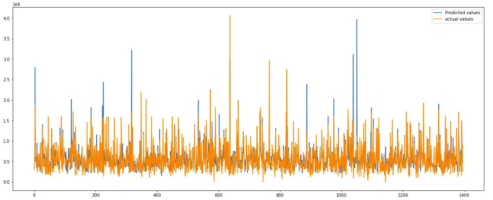
Although the plot shows the predictions were pretty good, it is difficult to compare it with the previous model. So, we will again find the R²-score.

# Evaluating the model
print('R score is :', r2_score(y_test, preds))

Output:

Notice that we’ve got a better R²-score value than in the previous model, which means the newer model has a better performance than the previous one.

Implementation of XGBoost for classification problem

A classification dataset is a dataset that contains categorical values in the output class. This section will use the digits dataset from the sklearn module, which has different handwritten images of numbers from 0 to 9. Each data point is an 8×8 image of a digit.

Importing and exploring the dataset

We have to import the dataset submodule of the sklearn module to get access to the digits dataset:

# importing the module
from sklearn import datasets
# loading dataset
dataset = datasets.load_digits()

Once we import the dataset, we can then start exploring it. Let’s first print out the keys of the dataset and see what kind of information we can get from there.

# dataset key values
dataset.keys()

Output:

You can explore each of the keys above on your own to see the kind of values they contain. Here, we will explore the key ‘DESCR’, which contains detailed information about the dataset.

# printing the information about dataset 
print(dataset['DESCR'])

Output:

Optical recognition of handwritten digits dataset
--------------------------------------------------
**Data Set Characteristics:**
    :Number of Instances: 1797
    :Number of Attributes: 64
    :Attribute Information: 8x8 image of integer pixels in the range 0..16.
    :Missing Attribute Values: None
    :Creator: E. Alpaydin (alpaydin '@' boun.edu.tr)
    :Date: July; 1998
This is a copy of the test set of the UCI ML hand-written digits datasets
https://archive.ics.uci.edu/ml/datasets/Optical+Recognition+of+Handwritten+Digits
The data set contains images of hand-written digits: 10 classes where
each class refers to a digit.
Preprocessing programs made available by NIST were used to extract
normalized bitmaps of handwritten digits from a preprinted form. From a
total of 43 people, 30 contributed to the training set and different 13
to the test set. 32x32 bitmaps are divided into nonoverlapping blocks of
4x4 and the number of on pixels are counted in each block. This generates
an input matrix of 8x8 where each element is an integer in the range
0..16. This reduces dimensionality and gives invariance to small
distortions.
For info on NIST preprocessing routines, see M. D. Garris, J. L. Blue, G.
T. Candela, D. L. Dimmick, J. Geist, P. J. Grother, S. A. Janet, and C.
L. Wilson, NIST Form-Based Handprint Recognition System, NISTIR 5469,
1994.
.. topic:: References
  - C. Kaynak (1995) Methods of Combining Multiple Classifiers and Their
    Applications to Handwritten Digit Recognition, MSc Thesis, Institute of
    Graduate Studies in Science and Engineering, Bogazici University.
  - E. Alpaydin, C. Kaynak (1998) Cascading Classifiers, Kybernetika.
  - Ken Tang and Ponnuthurai N. Suganthan and Xi Yao and A. Kai Qin.
    Linear dimensionalityreduction using relevance weighted LDA. School of
    Electrical and Electronic Engineering Nanyang Technological University.
    2005.
  - Claudio Gentile. A New Approximate Maximal Margin Classification
    Algorithm. NIPS. 2000.

Let’s print out the shape of the dataset and the images used in the dataset.

# printing the shape
print("shape of images is :", dataset.images.shape)
print("shape of dataset is:", dataset.data.shape)

Output:

Pay attention that the sizes of the images are 3X3 matrices, and the dataset is 2X2 matrices.

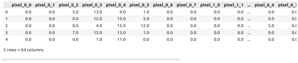
Let’s now print out the few rows from the data to see the kind of data points in our dataset.

# convertig the dataset into pandas dataframe
data = pd.DataFrame(dataset.data, columns=dataset.feature_names)
# printing the independent column
data.head()

Output:

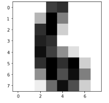
Images are just numbers in the form of matrices, so the about data represents the images. Now we will also print out any random image from the images.

# importing the module
import matplotlib.pyplot as plt
# printing the image of 6
plt.imshow(dataset.images[6], cmap=plt.cm.gray_r, interpolation='nearest')
plt.show()

Output:

Splitting the dataset

Before going to train the model on the dataset, we have to split the dataset into inputs and outputs.

# splitting the data into inputs and outputs
Input, output = datasets.load_digits(return_X_y=True)

The next step is to split the dataset into training and testing datasets so that we can evaluate the performance of the model after training.

# importing the module
from sklearn.model_selection import train_test_split
# splitting the dataset
X_train, X_test, y_train, y_test = train_test_split(Input, output, test_size=0.30)

We have assigned 30% of the dataset to the testing and the remaining 70% for the model’s training.

Training the model using the XGBoost classifier

Now we will train on the default parameter values. You can change these parameters values to get a better model or use the GridSearchCV to find the optimum parameters as explained above.

# Default parameters
xg_clf = xgb.XGBClassifier()
# training the model
xg_clf.fit(X_train,y_train)

Once the model is trained on the training dataset, we can use the testing data to predict the output class.

# testing the model
xgb_clf_preds = xg_clf.predict(X_test)

The next step is to see how well our model predicts the output class.

Evaluation of XGBoost classifier

We will use a confusion matrix and accuracy to evaluate the model’s evaluation. A confusion matrix is a table used to describe the performance of a classification model (or “classifier”) on a set of test data for which the valid values are known. It contains actual and predicted values.

Let’s now print out the confusion matrix of the XGBoost classifier.

# importing the modules
import seaborn as sns
from sklearn.metrics import confusion_matrix
# providing actual and predicted values
cm = confusion_matrix(y_test, xgb_clf_preds)
sns.heatmap(cm,annot=True)
# saving confusion matrix in png form
plt.savefig('confusion_Matrix.png')

Output:

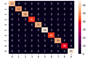
All the values from the colored diagonal are incorrectly classified, and we can see that there are very few of them. That means our model has performed very well on the given dataset.

Let’s now calculate the model’s accuracy as well.

# importing accuracy score
from sklearn.metrics import accuracy_score
# printing the accuracy score
accuracy_score(y_test,xgb_clf_preds)

Output:

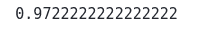
The output shows that our model has accurately classified 97% of the input data.

Additional Learning Materials

From our point of view, these are the best hands-on online courses related to Machine Learning and Deep Learning available on the market right now:

Summary

XGBoost is an algorithm that has recently dominated applied Machine Learning and Kaggle competitions for structured or tabular data. XGBoost implements Gradient Boosted Decision Trees designed for speed and performance. This article described the XGBoost algorithm and covered its implementation for solving classification and regression problems using Python.