K means clustering Python implementation example

Unsupervised Learning uses Machine Learning algorithms to analyze and cluster unlabeled datasets and discover hidden patterns or data groupings without human intervention. There are two types of Unsupervised Learning algorithms: Clustering and Association Rules. The K means clustering (Python) algorithm belongs to the clustering methods of Data Science.

This article contains the K means clustering Python implementation and visualization examples for data classification.

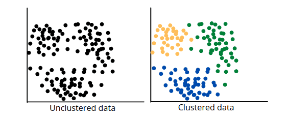
Clustering is one of the most common exploratory data analysis techniques to understand the data structure. Clustering algorithms allow you to discover homogeneous subgroups within the dataset so that data points in each cluster of initial centroids are comparable and similar based on a similarity measure like euclidean or correlation-based distance.

K-mean clustering algorithm overview

The K-means is an Unsupervised Machine Learning algorithm that splits a dataset into K non-overlapping subgroups (clusters). It allows us to split the data into different groups or categories. For example, if K=2 there will be two clusters, if K=3 there will be three clusters, etc. Using the K-means algorithm is a convenient way to discover the clusters of assignments or categories of groups in the unlabeled dataset with all the data points.

The K-means algorithm (also known as a centroid-based algorithm) aims to minimize the sum of distances between the data point and their corresponding clusters while associating each group of objects called a cluster centroid, a (cluster) with its centroid.

The K-means algorithm does two things:

• Iteratively determines the best value for centroids (center points for every K’s cluster, which can also be called k centroids)
• Assigns each data point to its closest K-center. The nearest K-center data points form a cluster.

As a result, each cluster will have data points with similar features:

The K-means algorithm description:

1. Define the number of clusters based on provided K value
2. Select random K points or centroids (can differ from the input dataset)
3. Form the K clusters by assigning each data point to their closest centroid
4. Calculate the variance and define new centroids of each cluster
5. Repeat the process from the third step to reassign each datapoint with centroid initialization to the new closest centroid of each cluster until the algorithm finds the best possible solution

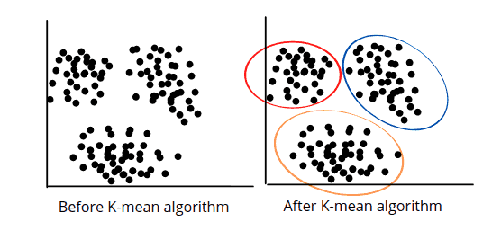
Let’s visualize the steps involved after the clustering step in the training of the K-mean clustering algorithm.

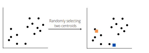
Suppose that we have plotted data, and we want to apply the K-means algorithm to find out the clusters/hidden patterns. Let’s, for example, split the dataset into two different clusters (K=2). The algorithm will choose random points K for each centroid to form the cluster. These points can be either the points from the dataset or any other points. Let’s say the algorithm selects the following two centroids:

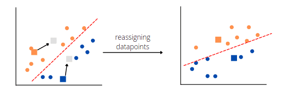
Next, the algorithm will assign each data point to its closest centroid and compute the distance between the data points and the cluster center of the centroids to define the median between the two clusters:

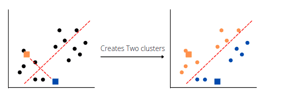
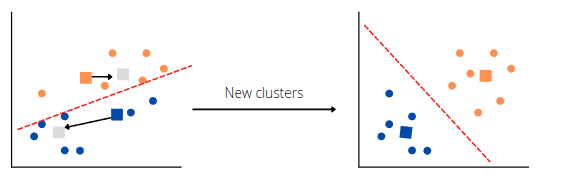
Next, the K-means clustering algorithm will choose new centroids based on each cluster’s calculated center of gravity, reassign each datapoint to the new centroid, and find a median for new clusters:

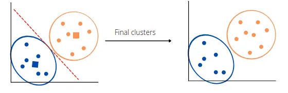
The exact process will repeat until the algorithm finds the optimum clusters:

Finally, the algorithm will split all data points from the dataset into the best possible clusters or groups:

Elbow method: Getting the value of K

The K-means clustering algorithm’s performance is highly dependent on the number of clusters, and choosing the correct value for K of the K groups is very important but might be challenging. You can use the Elbow method to calculate the ideal number of clusters in the dataset.

The Elbow method uses the Within Cluster Sum of Squares (WCSS) value to define total variations. Here’s a simple formula for two clusters:

The equation ∑Pi in Cluster1 distance(Pi C1)2 represents the sum of the squares of the distances (Euclidean distance or the Manhattan distance) between each data point and its cluster’s centroid.

The following steps calculate the optimal value for K:

• For various K values, use the K-means clustering to split the dataset
• Calculate the WCSS value For each K
• It will then plots a curve graph between calculated WCSS values and the number of clusters K
• The sharp point of bend or a point of the plot that looks like an arm is the best value for K

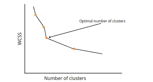
One of the limitations of the Elbow method is that it doesn’t always work well, primarily when it is hard to split data points into clusters and because of the dimensionality reduction shown in the graph above. We’ll show this case in the next section.

When the K-means algorithm produces incorrect results

As soon as we describe the concepts of the K-means and Elbow method, let’s try to apply them to the real dataset and use Python to solve the classification problem with the python implementation.

We’ll use the Facebook Live Sellers in Thailand DataSet, which you can download here, and the following Python modules for the implementation and visualization:

• pandas
• sklearn
• numpy
• matplotlib
• seaborn

You can install them in your AWS Sagemaker Jupyter Notebook by running the following commands in its cell:

%pip install pandas
%pip install sklearn
%pip install numpy
%pip install matplotlib
%pip install seaborn

Exploring and cleaning the dataset

We will use the pandas module and its pd.read_csv() method to import our input data from the dataset:

# importing the module
import pandas as pd
# importing the dataset
data = pd.read_csv("K-Means-dataset.csv")

Let’s get the shape of the dataset:

# shape of the dataset
print(data.shape)

Output:

The output shows 7050 records in the dataset (each record contains 16 attributes).

The description of the dataset contains information that the dataset contains 7051 records with 12 attributes per record. Let’s dive deep into data.

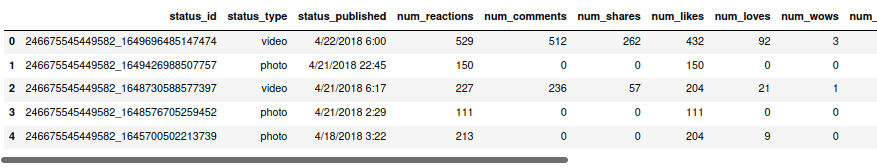
Let’s preview that dataset by using the head() method:

# previewing the dataset
data.head()

Output:

Next, we can check for the missing values in the dataset. Pandas provide us with a built-in method isnull(), which will help us to identify the missing values:

# printing the missing values
print(data.isnull().sum())

Output:

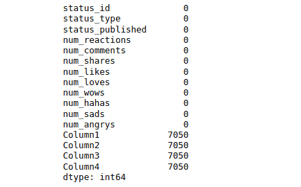
The output shows that the last four-column contain 7050 null values. These columns are useless, so let’s delete them from the dataset:

# droping the columns with missing values
data.drop(['Column1', 'Column2', 'Column3', 'Column4'], axis=1, inplace=True)
# checking null values
print(data.isnull().sum())

Output:

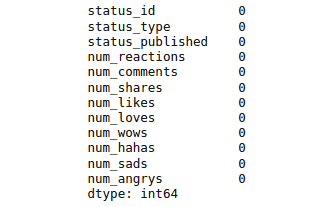
We used the inplace to modify the original dataset with the new data instead of making its copy.

Let us now use the info() method to get more information about the types of data each attribute has.

# getting info about data
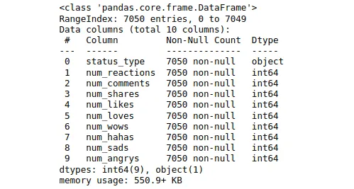
data.info()

Output:

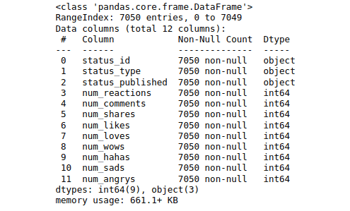
The output shows three columns with string values (object in the Dtype column) and nine numerical columns (int64 in the Dtype column) in the dataset.

Now let us explore each column with string values one by one.

First, let’s take a look at the status_id variable:

# labels in the variable
unique_data = data['status_id'].unique()
# printing total uniques values
print (len(unique_data))

Output:

The output from the above code shows that there are 6997 unique labels in the status_id column. The total number of instances in the dataset is 7050. So, it might be a unique identifier for each record in the dataset, which we can’t use for clustering. So we need to delete it from our dataset too:

# droping the status id variable from data set
data.drop(['status_id'], axis=1, inplace=True)

Next, let’s take a look at the status_published column:

# labels in the variable
unique_data = data['status_published'].unique()
# printing total uniques values
print (len(unique_data))

Output:

The output shows 6913 unique out of 7050 records in this column. We can’t use this column for clustering too. Let’s drop it:

# droping the status publisehd variable from data set
data.drop(['status_published'], axis=1, inplace=True)

Let us now explore the last string column (status_type):

# labels in the variable
unique_data = data['status_type'].unique()
# printing total uniques values
print (len(unique_data))

Output:

The output shows that there are only four unique labels in the status_type column, so we can keep it.

Let’s again use the info() method to see the details about the dataset:

# info about data set
data.info()

Output:

The output shows that there is now only one column with non-numeric values.

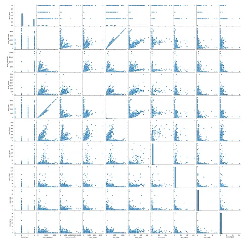
We can use the seaborn module and the pairplot graph to visualize data correlation in the dataset:

# ploting the pairplot graph
sns.pairplot(data)

Output:

As soon as the K-means algorithm requires numeric data as input, let’s replace the status_type column values with the numeric values:

# feature vector
X = data
# target variable
y = data['status_type']
# importing label encoder
from sklearn.preprocessing import LabelEncoder
# converting the non-numeric to numeric values
le = LabelEncoder()
X['status_type'] = le.fit_transform(X['status_type'])
y = le.transform(y)

If we print the dataset, we will see numeric values under the status_type variable:

# printing the dataset
X.head()

Output:

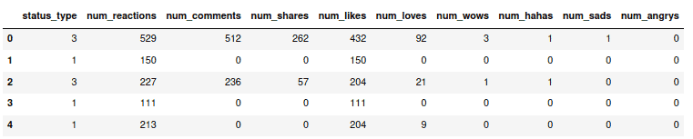
Note: values of the status_type column has been changed to discrete numeric values.

Splitting the dataset into two clusters

Now, let’s find relationships between items in the dataset and how many clusters should be in the dataset using the sklearn K-mean class with K=2.

# importing k-mean
from sklearn.cluster import KMeans
# k value assigned to 2
kmeans = KMeans(n_clusters=2, random_state=0) 
# fitting the values
kmeans.fit(X)
# Cluster centers
kmeans.cluster_centers_

Output:

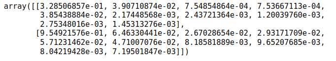
The K-Means algorithm creates clusters from data with only a single cluster by separating samples in n groups of equal variances, minimizing a criterion known as inertia.

Inertia measures how well a dataset was clustered by K-Means. It is calculated by measuring the distance between each data point and its centroid, squaring this distance, and summing these squares across one cluster.

Clustering: K-Means

The K-means algorithm chooses cluster centroids that minimize the inertia value. So one way to evaluate the K-mean algorithm is to check whether the inertia is small or large. The smaller the inertia value will be, the better the algorithm performs.

So, let’s print the inertia value and check the algorithm’s performance for 2 clusters:

# printing the value of inertia
print (kmeans.inertia_)

Output:

We get a very high value for the inertia, which means our model is not performing well.

Let’s check how many data points have been classified correctly.

# stroing labels
labels = kmeans.labels_
# check how many of the samples were correctly labeled
correct_labels = sum(y == labels)
# printing the results
print("Result: %d out of %d samples were correctly labeled." % (correct_labels, y.size))

Output:

The output proves that the algorithm did not work well, and we need to change the number of clusters to get better results.

Splitting the dataset into three clusters

For our dataset, the K-means algorithm did not work well for two clusters (K=2). Let’s try to increase the value of K to K=3.

# importing k-mean
from sklearn.cluster import KMeans
# k value assigned to 2
kmeans = KMeans(n_clusters=3, random_state=0) 
# fitting the values
kmeans.fit(X)
# Cluster centers
kmeans.cluster_centers_
# printing the value of inertia
print (kmeans.inertia_)

Output:

The inertia value is lower than in the previous attempt, which means the model performed better than last time when the value of the K was 2.

Let’s check the quality of the classification:

# stroing labels
labels = kmeans.labels_
# check how many of the samples were correctly labeled
correct_labels = sum(y == labels)
# printing the results
print("Result: %d out of %d samples were correctly labeled." % (correct_labels, y.size))

Output:

This time our model performed better but not enough. We need to change the value of K to get better results.

Using the Elbow algorithm to get a better K value

Instead of iterating over different values for K manually, we can plot the Elbow algorithm results and get the optimal value for K from the graph.

# Using the elbow method to find the optimal number of clusters
from sklearn.cluster import KMeans
# to store WCSS
wcss = []
# for loop 
for i in range(1, 11):
    
    # k-mean cluster model for different k values
    kmeans = KMeans(n_clusters = i, init = 'k-means++', random_state = 42)
    kmeans.fit(X)
    
    # inertia method returns wcss for that model
    wcss.append(kmeans.inertia_)
    
# importing the matplotlib module
import matplotlib.pyplot as plt
# figure size
plt.figure(figsize=(10,5))
sns.lineplot(range(1, 11), wcss,marker='o',color='green')
# labeling
plt.title('The Elbow Method')
plt.xlabel('Number of clusters')
plt.ylabel('WCSS')
plt.show()

Output:

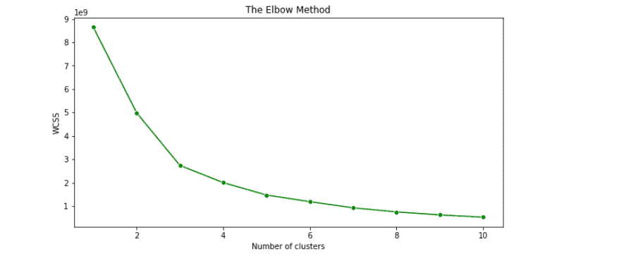
As you can see, the graph shows that we can use K=3 for the K-Means algorithm, but we failed to get the correct results because we’re dealing with categorical data.

Visualizing dataset clusters

Let’s look at centroids/data distribution for the K=3.

# k-mean algorithm
kmeans = KMeans(n_clusters = 3, random_state = 42)
y_kmeans = kmeans.fit_predict(X)
X = np.array(X)
# size of image
plt.figure(figsize=(15,7))
# visualizing the clusters
sns.scatterplot(X[y_kmeans == 0, 0], X[y_kmeans == 0, 1], color = 'yellow', label = 'Cluster 1',s=50)
sns.scatterplot(X[y_kmeans == 1, 0], X[y_kmeans == 1, 1], color = 'blue', label = 'Cluster 2',s=50)
sns.scatterplot(X[y_kmeans == 2, 0], X[y_kmeans == 2, 1], color = 'green', label = 'Cluster 3',s=50)
sns.scatterplot(kmeans.cluster_centers_[:, 0], kmeans.cluster_centers_[:, 1], color = 'red', 
                label = 'Centroids',s=300,marker=',')
# labeling
# plt.grid(False)
plt.title('Three clusters')
plt.xlabel('Status_type')
plt.ylabel('values')
plt.legend()
plt.show()

Output:

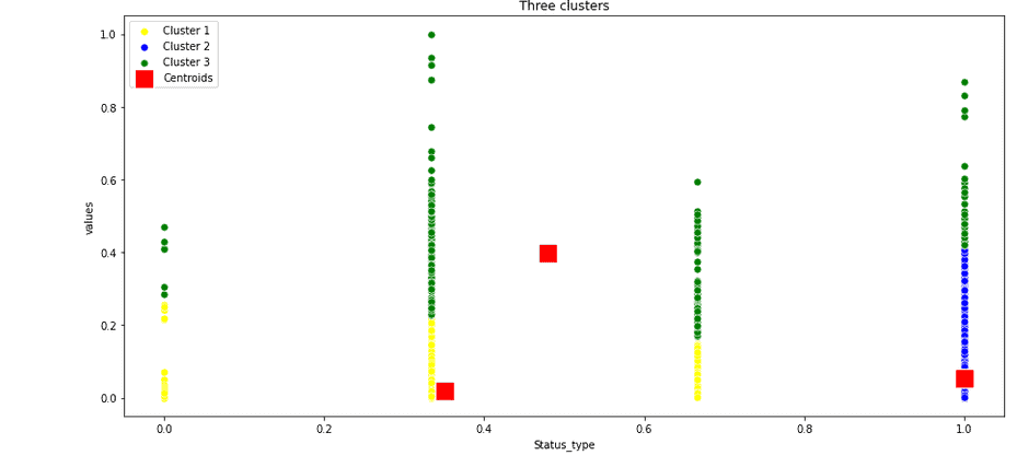
The chart shows that we’re dealing with categorical data distribution based on the status_type column values, and the K-means clustering algorithm fails to perform well because the values from the status_type column does not correlate with other columns’ values.

K Means clustering Python algorithm for data classification

Let’s take a different dataset that contains information about the mall’s customers. You can get access to the dataset here.

In this example, we’ll be interested in segmenting customers’ info (separating customers into groups based on their sales, needs, etc.). This segmentation might improve relationships between the company and its customers.

Now, we’ll implement K means clustering in Python. Let’s quickly walk through the dataset:

# importing dataset
dataset2 = pd.read_csv("k-mean-dataset-mall-customer.csv")
# printing the info about dataset
dataset2.info

Output:

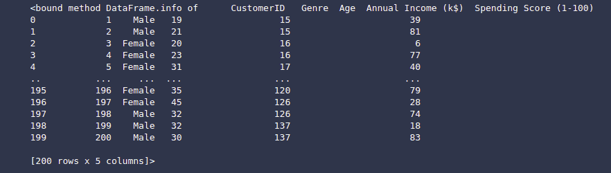
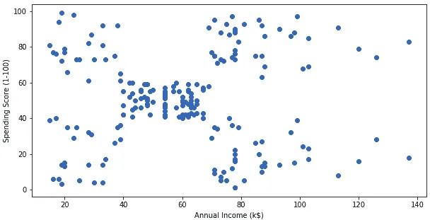
For simplicity, let’s take two attributes and build a scattered graph to confirm that our data is well dispersed.

# stroing two attributes
X = dataset2.loc[:, ['Annual Income (k$)', 'Spending Score (1-100)']]
# importing the module
import matplotlib.pyplot as plt 
# image size
plt.figure(figsize=(10,5))
# ploting scatered graph
plt.scatter(x= X['Annual Income (k$)'], y=X['Spending Score (1-100)'])
plt.xlabel('Annual Income (k$)')
plt.ylabel('Spending Score (1-100)');

Output:

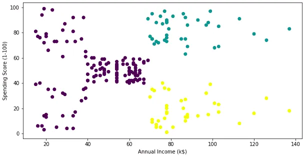
Splitting the dataset into three clusters

Let’s use the K-Means algorithm to split customers into three (K=3) categories of cluster labels.

# importing the k-means
from sklearn.cluster import KMeans
# cluster size is set to be 3
km = KMeans(n_clusters = 3)
km.fit(X)
# ploting the graph of the clusters
plt.figure(figsize=(10,5))
plt.scatter(x= X.iloc[:, 0], y=X.iloc[:, 1], c= km.labels_)
plt.xlabel('Annual Income (k$)')
plt.ylabel('Spending Score (1-100)');

Output:

Looks good, but you will get a different result if you start playing with the random_state variable:

# ploting graph in one line
fig, ax = plt.subplots(1, 3, gridspec_kw={'wspace': 0.3}, figsize=(15,5))
# build three graphs
for i in range(3):
    km = KMeans(n_clusters = 3, init='random', n_init=1, random_state=i)
    km.fit(X)
    ax[i].scatter(x= X.iloc[:, 0], y=X.iloc[:, 1], c= km.labels_);

Output:

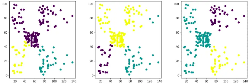
 As you can see from the graphs, we’re getting different results when we run the K-means algorithm and shuffle the data. So it would be better to split the dataset into a different number of clusters to its nearest centroid.

Evaluating the K-Mean algorithm using inertia

The section above showed that the K-Means algorithm produced different results from the same dataset with shuffled data. So, how could we know which graph is more efficient? We need to use inertia. The lower the value of inertia, the better the algorithm performed.

Let’s look at which of the graphs has the lowest inertia value.

# creating graph in one line
fig, ax = plt.subplots(1, 3, gridspec_kw={'wspace': 0.3}, figsize=(15,5))
# for loop 
for i in range(3):
    km = KMeans(n_clusters = 3, init='random', n_init=1, random_state=i)
    km.fit(X)
    ax[i].scatter(x= X.iloc[:, 0], y=X.iloc[:, 1], c= km.labels_)
#     printing the interia with graphs
    ax[i].set_title(f"Inertia = {round(km.inertia_, 2)}");

Output:

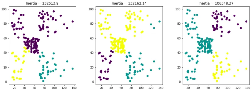
The output shows that the last graph is more efficient as it has the lowest inertia score among the three.

Finding the optimal number of clusters

Let’s use the Elbow method to find the optimal number of clusters for the given dataset.

# Within cluster sum squares
wcss = [] 
# for loop
for i in range(2,15):
    km = KMeans(n_clusters= i)
    km.fit(X)
    wcss.append(km.inertia_)
    
# ploting the elbow graph
plt.plot(range(2,15), wcss, 'og-')
plt.annotate('Elbow', xy=(5, 50000), xytext=(6, 100000), arrowprops=dict(facecolor='green', shrink=0.05))
plt.xlabel("K")
plt.ylabel("Inertia");

Output:

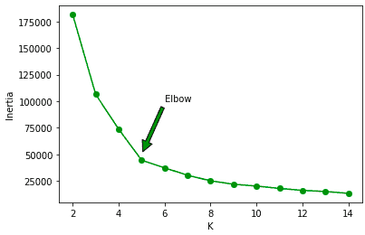
Note: the K-mean algorithm performed well when the number of clusters was five.

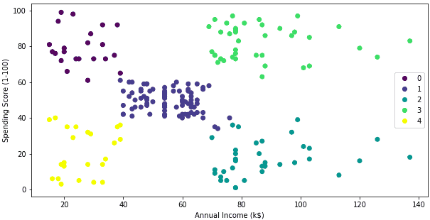
Splitting the dataset into five clusters

Let’s plot the classification results of our dataset from a scatter plot into five clusters.

# k mean algorithm training
km = KMeans(n_clusters = 5)
km.fit(X)
# ploting the graph
plt.figure(figsize=(10,5))
scatter = plt.scatter(x= X.iloc[:, 0], y=X.iloc[:, 1], c= km.labels_)
plt.xlabel('Annual Income (k$)')
plt.ylabel('Spending Score (1-100)')
# creating the labels for different clusters
plt.legend(handles=scatter.legend_elements()[0], labels=[0, 1, 2, 3, 4]);

Output:

FAQ

Summary

K-means clustering algorithm is a type of Unsupervised Learning used to split unlabeled data into several categories. The Elbow method allows you to find your dataset’s optimal number of clusters. This article covered the implementation and visualization of the K-means clustering algorithm and Elbow method using Python.