Neural Network Classification – Simple example

An Artificial Neural Network (ANN) is a computer model similar to the human brain. It comprises a set of interconnected processing nodes or neurons that can “interact” with each other. ANN can learn from data and make predictions based on patterns they identify in that data (solve classification problems).

TensorFlow is a free and open-source platform for Machine Learning (ML), offering a wide range of features that make it ideal for developing and training large-scale ML models.

This tutorial will demonstrate using TensorFlow to build a Neural Network classification model. First, we will create a deep learning model for binary classification, then move to multiclass classification. Finally, we will improve the model’s performance by tuning parameters.

We assume you have a basic understanding of Neural networks and TensorFlow. You can also check the articles: Introduction to Neural Networks and Introduction to Tensorflow to refresh your mind.

Getting started with Neural Network Classification

As we know, a classification problem is a problem having categorical output values. In the case of binary classification, the output class contains only two categories, and in the case of a multi-classification problem, the output class has more than two categories.

The neural network’s architecture for binary classification looks very similar to the neural network for regression one. However, the activation function on the output layer should be sigmoid in the case of binary classification,

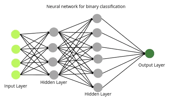
You can apply any activation function(except softmax) to the hidden layers. Still, the activation function on the output layer should be sigmoid as the sigmoid functions give the probability (between 0 and 1).

The architecture of neural networks for multiclass classification is similar to the binary one, except that the nodes in the output layer are equal to the output categories. For example, if our data set contains information about four different types of animals (output has 4 categories), then the neural network will be:

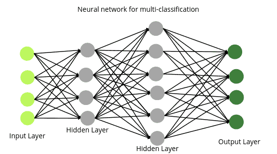
Similar to any other neural network, you can apply any activation function on the hidden layers, but in the case of a multiclass problem, the activation function on the output layer should be softmax as it gives us the probability for multi-items.

Neural Network for Binary classification using TensorFlow

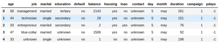
Now, we will use TensorFlow to create a model in neural networks to solve a binary classification. The dataset that we will be using contains information about bank marking campaigns based on phone calls. The output class includes whether or not the clients will subscribe to their services. You can read more about the dataset and download it from this link.

Before going to the implementation part, ensure you have installed the following Python libraries on your system.

• TensorFlow
• sklearn
• pandas
• matplotlib
• seaborn

You can install the required modules by running the following commands in the cell of the Jupyter notebook.

%pip install tensorflow
%pip install sklearn
%pip install pandas
%pip install matplotlib
%pip install seaborn

Once these modules are installed successfully, we can move to the implementation part.

Importing and exploring the dataset

We will import the dataset and print out a few rows using the Pandas module.

# importing pandas module
import pandas as pd
# importing dataset
data = pd.read_csv('bank-full.csv', sep=';')
# heading
data.head()

Output:

Next, let us use the info() method to find more information about the dataset.

# printing info dataset
data.info()

Output:

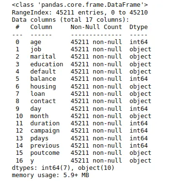
Notice that we have 45211 observations, and most columns are object types. We will now use the LabelEncoding method to change the typed object values into numeric ones.

# importing the module
from sklearn import preprocessing
  
# creating labing encoding object
label_encoder = preprocessing.LabelEncoder()
  
# Encode labels in multiple columns
data['job']= label_encoder.fit_transform(data['job'])
data['marital']= label_encoder.fit_transform(data['marital'])
data['education']= label_encoder.fit_transform(data['education'])
data['default']= label_encoder.fit_transform(data['default'])
data['housing']= label_encoder.fit_transform(data['housing'])
data['housing']= label_encoder.fit_transform(data['housing'])
data['loan']= label_encoder.fit_transform(data['loan'])
data['contact']= label_encoder.fit_transform(data['contact'])
data['month']= label_encoder.fit_transform(data['month'])
data['poutcome']= label_encoder.fit_transform(data['poutcome'])
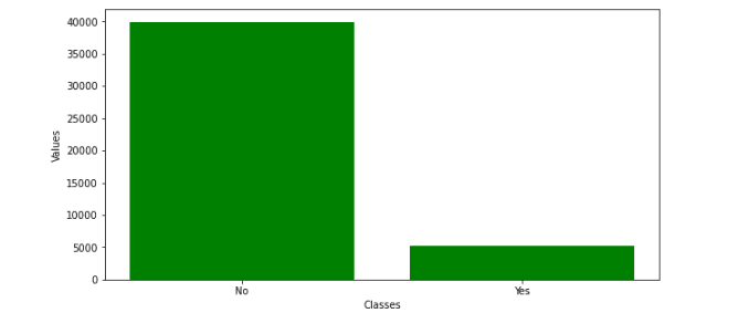
data['y']= label_encoder.fit_transform(data['y'])

Let us plot the bar chart for the output values using Matplotlib:

# importing matplotlib
import matplotlib.pyplot as plt
# plotting
fig = plt.figure(figsize = (10, 5))
#  Bar plot
plt.bar(['No',"Yes"], data.y.value_counts(), color ='green',
        width = 0.8)
# labeling
plt.xlabel("Classes")
plt.ylabel("Values")
plt.show()

Output:

Splitting dataset

Now, we will divide the dataset into input values and output classes.

# splitting dataset
X = data.drop('y', axis=1)
y = data['y']

Let us now split the dataset set input testing and training data.

# importing the module
from sklearn.model_selection import train_test_split
# splitting into training data and test dataset 
X_train, X_test, y_train, y_test = train_test_split(X, y, test_size=0.30, random_state=1)

As you can see, we have assigned 70% of the data to the training and the remaining 30% to the testing.

Building neural network model for binary classification using TensorFlow

Now, we will use TensorFlow to build a neural network for binary classification.

# importing required module
from tensorflow.keras.layers import Dense
from tensorflow.keras.layers import InputLayer
from tensorflow.keras import Sequential
# defining neural network model
model = Sequential()
# adding input layer with 16 nodes
model.add(InputLayer(16))
# adding hidden layer with 10 nodes
model.add(Dense(10, activation='relu', kernel_initializer='he_normal'))
# adding output layer to neural network model
model.add(Dense(1, activation='sigmoid'))

The above code will create a neural network similar to the below one:

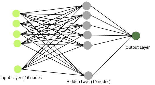
Notice that we have assigned 16 nodes to the input layer as our dataset contains 16 independent variables. We also added one hidden with 10 nodes and applied the ReLU activation function on it( you can increase the hidden layers and change the number of nodes to achieve better results, but make sure your model will not overfit). Moreover, the number of nodes in the output layer is 1, and the activation function is sigmoid, as we deal with binary classification problems.

The next step is to compile the model.

# compile the model with loss function binary_crossentropy
model.compile(optimizer='adam', loss='binary_crossentropy', metrics=['accuracy'])

As you can see, we have used Adam as an n-optimizer and binary_crossentropy as the loss function. The binary_crossentropy function is used in binary classification and computes the cross-entropy loss between true and predicted labels.

Now, it is time to train the model using the training dataset.

# fit the model
model.fit(X_train, y_train, epochs=50)

We have fixed the number of epochs to 50. An epoch means training the neural network with all the training data for one cycle. You can change the number of epochs to get an optimum solution.

Evaluating the trained model

Now we will use the testing data to evaluate the model’s performance. Let us use the testing data to make predictions using our trained model and evaluate the model.

# evaluate the model with test dataset
evaluate = model.evaluate(X_test, y_test)
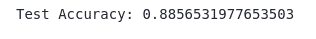
print('Test Accuracy:', evaluate[1])

Output:

The above output shows that our model could correctly classify 85% of the testing dataset.

Parameter tuning to find the optimum number of nodes and epochs

Now, we will learn how to find the optimum number of nodes in the hidden layer and epoch value. We will use the Keras parameter tunning method known as Hyperband tunning.

We will first create a function that will initialize our model for binary classification with a maximum and a minimum number of nodes in the hidden layer.

# importing the module
from tensorflow import keras

# function to create model
def model_builder(hp):
    
#     initializaing the classification model
    model = keras.Sequential()
    model.add(InputLayer(16))
#     specifying the maximum and minimum nodes
    hp_units = hp.Int('units', min_value=5, max_value=100)
    model.add(keras.layers.Dense(units=hp_units, activation='relu'))
    model.add(keras.layers.Dense(1, activation='sigmoid'))
#     comppiling the model with loss function binary crossentropy
    model.compile(optimizer='adam',
                    loss='binary_crossentropy',
                    metrics=['accuracy'])
#   return classification model
    return model

Let us initialize the hyperband tunning from the Keras module.

# importing the module
import keras_tuner as kt
import tensorflow as tf
# calling the function using hyperband 
tuner = kt.Hyperband(model_builder,
                     objective='val_accuracy',
                     max_epochs=100)

The Hyperband tuning algorithm uses adaptive resource allocation and early stopping to converge quickly on a high-performing model. It ensures that our model is not overfitted and stops the iterations once a specified result is achieved.

# early stopping
stop_early = tf.keras.callbacks.EarlyStopping(monitor='val_loss', patience=5)

We will start the tuner search and find the optimum number of nodes in the hidden layer.

# initializing the tunner
tuner.search(X,y, epochs=100, validation_split=0.2, callbacks=[stop_early])
# Get the optimal hyperparameters
best_hps=tuner.get_best_hyperparameters(num_trials=1)[0]
print("Optimin number of nodes in hidden layer are :", best_hps.get('units'))

Output:

As you can see, the optimum number of nodes in the hidden layer is 54. Now, let us also find the optimum number of epochs using the parameters returned by the tuner search.

# creating model with optimimum parameters
model = tuner.hypermodel.build(best_hps)
# model training
history = model.fit(X, y, epochs=200, validation_split=0.2)
# fining the optimum epochs
val_acc_per_epoch = history.history['val_accuracy']
best_epoch = val_acc_per_epoch.index(max(val_acc_per_epoch)) + 1
print('Best epoch value is: ' ,best_epoch)

Output:

As you can see, the tuner has returned 38 as the optimum value for the model.

Training the model with optimum parameters

Now, we will use optimum numbers returned by the Keras tuner for several nodes and epochs to train the model and see the result.

# define model
model = Sequential()
# adding input layer with 16 nodes
model.add(InputLayer(16))
# adding hidden layer with 10 nodes
model.add(Dense(54, activation='relu', kernel_initializer='he_normal'))
# adding output layer 
model.add(Dense(1, activation='sigmoid'))
# compile the model
model.compile(optimizer='adam', loss='binary_crossentropy', metrics=['accuracy'])
# model trained
model.fit(X_train, y_train, epochs=38)

# evaluate the model with accuracy metrics
evaluate = model.evaluate(X_test, y_test)
print('Test Accuracy:', evaluate[1])

Output:

As you can see, this time, we got an accuracy score of 88%, which means our model has performed a little better than the previous one, where we get an accuracy of 85%.

Multiclass classification using TensorFlow

Now, we will use TensorFlow for multiclass classification using Neural networks. In this section, we will use a dataset from a higher education institution related to students enrolled in different undergraduate degrees, such as agronomy, design, education, nursing, journalism, management, social service, and technologies. The data is used to build classification models to predict students’ dropout and academic success. So, there are three output categories; enrolled, dropout, and graduate. You can read about the dataset and download it from this link.

Importing and exploring the dataset

First, we import the dataset and print a few rows to familiarize ourselves.

# importing the dataset
dataset = pd.read_csv('dataset.csv', sep=";")
# heading of dataset
dataset.head()

Output:

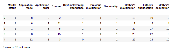
As you can see, there is a total of 35 columns and 34 of which are input variables. Let us also use the info() method to get more information about the dataset.

#info method
dataset.info()

Output:

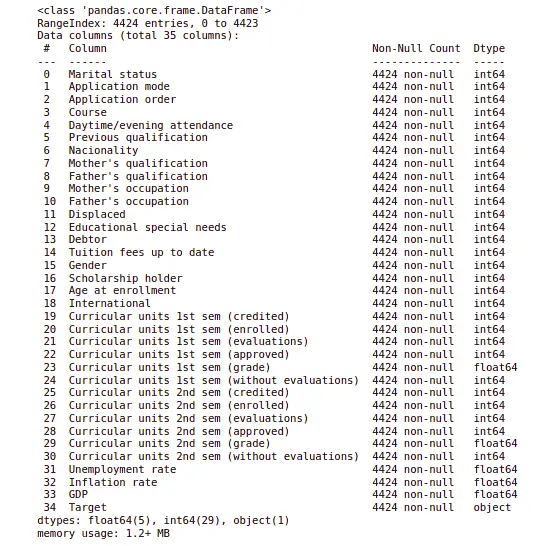
As you can see, our dataset contains 4424 observations, all of which have numeric values except the output class. So, let us now convert the object type object into numeric values.

# importing the module
from sklearn import preprocessing
  
# creating labing encoding object
label_encoder = preprocessing.LabelEncoder()
  
# Encode labels in multiple columns
dataset['Target']= label_encoder.fit_transform(dataset['Target'])

Now, the data is ready to be used to train the model

Splitting the dataset

Now, we will divide the dataset into input variables and output variables.

# dividing the dataset
X = dataset.drop('Target', axis=1)
y=dataset['Target']

The next step is to split the data into the testing and training parts.

# splitting the dataset 
X_train, X_test, y_train, y_test = train_test_split(X, y, test_size=0.25, random_state=1)

As you can see, we have assigned 25% of the dataset to the testing part and the remaining 75% to the training part.

Building Neural Network for multiclass classification

Let us initialize the model with the input, hidden, and output layers.

# define model
model = Sequential()
# adding input layer with 34 nodes
model.add(InputLayer(34))
# adding hidden layer with 10 nodes
model.add(Dense(10, activation='relu', kernel_initializer='he_normal'))
# adding output layer 
model.add(Dense(3, activation='softmax'))

The above code will create a neural network similar to the following image:

As you can see, the neural network has 34 nodes in the input layer ( as we have 34 independent variables). We have also assigned 10 nodes along with the ReLU activation function to the hidden layer. And finally, we have an output layer that contains three nodes ( as there are three output categories ), and the activation function on the output layer is softmax.

Let us now compile and train the model on the training dataset.

# compile the model
model.compile(optimizer='adam', loss='sparse_categorical_crossentropy', metrics=['accuracy'])
# fit the model
model.fit(X_train, y_train, epochs=50)

As you can see, we have used spare_categorical_crossentropy as our loss. Training a neural network involves passing data through the model and comparing predictions with ground truth labels. A loss function makes this comparison, and in the case of the multiclass classification problem, we used spare_categorical_crossentropy. We also fixed the epoch value to 50. You can change it to get optimum results.

Let us evaluate the model by testing and finding the accuracy score.

# evaluate the model
evaluate = model.evaluate(X_test, y_test)
# printing evaluate accuracy
print('Test Accuracy:', evaluate[1])

Output:

As you can see, we get an accuracy score of 76%, which means the model predicts 76% of the testing data correctly.

You can use the tunning parameter method to find the optimum parameters to get better results, as we did in the above section.

Summary

Neural networks are a series of algorithms that mimic the operations of a human brain to recognize relationships between vast amounts of data. You can use them for classification, regression, image recognition, forecasting, marketing research, and many more. This article taught us how to use TensorFlow to build a neural network to solve a binary and multiclass classification problem.