Introduction to TensorFlow

TensorFlow is a sophisticated Machine Learning software library created by Google. It allows creating custom algorithms for various purposes, including image and video recognition, natural language processing, and predictive analytics. TensorFlow can also run on various platforms, including CPUs, GPUs, and TPUs. It provides an extensive API that makes developing complex Machine Learning models easy. In addition, TensorFlow offers several high-level APIs that make it possible to develop and train models quickly. This is the first article for the TensorFlow tutorials, and it supposes to help you get started with TensorFlow, its installation, and its basic features.

TensorFlow can train and run deep learning models for handwritten digit classification, image recognition, word embeddings, recurrent neural network, sequence-to-sequence models for machine translation, natural language processing, and PDE (partial differential equation) based simulations. Before starting this article about Tensoflow, ensure you have a basic understanding of Neural networks. You can read about Artificial Neural networks in the article, Introduction to Artificial Neural Network.

What is TensorFlow?

TensorFlow is a powerful and popular open-source software library designed for numerical computation using data flow graphs. TensorFlow was originally developed by researchers and engineers working on the Google Brain team within Google’s Machine Intelligence research organization to meet the demand for faster and more efficient Deep Learning algorithms. TensorFlow is used by major organizations such as Airbus, NVIDIA, Twitter, Yahoo, DropBox, and many others.

It has been ported to several platforms, including JavaScript and iOS. TensorFlow.js is an open-source library that can train and deploy Machine Learning models in the browser. TensorFlow Lite is a production-ready solution for mobile devices that enables on-device machine learning inference. TensorFlow Extended (TFX) is a platform for developing and deploying production-scale Machine Learning pipelines. TFX was designed to be used with TensorFlow models but can also be used with other machine learning frameworks such as XGBoost and scikit-learn.

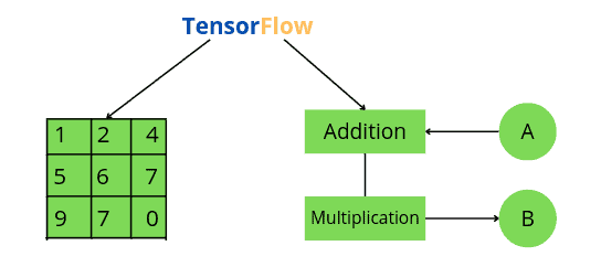
TensorFlow is made of two words, i.e., Tensor and Flow, where the “Tensor” is simply a multidimensional array, and the “Flow” is used to define the flow of data in operation.

Features of TensorFlow

The following are some of the popular features of TensorFlow that you should know:

• TensorFlow is an open-source library that allows rapid and easier calculations in machine learning.
• We can execute TensorFlow applications on platforms such as Android, Cloud, iOS, and various architectures such as CPUs and GPUs. This allows it to be executed on various embedded platforms.
• TensorFlow has its own designed hardware to train the neural models known as Cloud TPUs (TensorFlow Processing Unit).
• TensorFlow provides a fast debugging method. Tensor Board works with the graph to visualize its working using its dashboard.
• It works with multidimensional arrays with the help of a data structure tensor which represents the edges in the flow graph.
• TensorFlow provides a defined level of abstraction by reducing the code length and cutting the development time.
• TensorFlow provides the process of resolving complex topologies with the support of Keras API and data input pipelines.
• TensorFlow offers pipelining because you can train multiple neural networks and GPUs, making the models very efficient on large-scale systems.
• We can easily build and train ML models using intuitive high-level APIs like Keras with eager execution, which makes for immediate model iteration and easy debugging.

Applications of TensorFlow

As we discussed earlier, the major uses of the Tensorflow library include deep learning models for classification, perception, understanding, discovery, prediction, and creation. Here we will look at some of the real-life applications of TensorFlow.

• DeepSpeech is an automatic speech recognition (ASR) engine that aims to make speech recognition technology and trained models available to developers. It has been implemented in TensorFlow.
• Another implementation of TensorFlow is RankBrain, developed by Google and is a large-scale deployment of deep neural nets for search ranking on Google. It is a part of the search algorithm used to sort through the billions of pages and find the most relevant ones.
• Another application of TensorFlow is the Massive multitask for Drug Discovery developed by Stanford University, a deep neural network model for identifying promising drug candidates.
• Using TensorFlow, we can make algorithms to paint an image or visualize objects in a photograph. We can also train a PC to recognize objects in an image and use that data to drive new and interesting behaviors.
• Using TensorFlow, we can even teach the computer to read and synthesize new phrases, which is part of Natural Language Processing.
• Machine learning has great use in recommendation engines, and almost every big company uses it in some form. TensorRec is another cool recommendation engine framework in TensorFlow, which has an easy API for training and prediction.
• Image recognition is one of the most popular uses of TensorFlow, which is used by many mobile companies, social media, and other telecom houses.
• Another important application of TensorFlow is Video detection.

Getting started with the basics of TensorFlow

Now we will jump into the practical part of TensorFlow, where we will learn how to install and explore some basic operations.

Before starting, make sure that you have Python installed on your system. If not, you can download the updated version of Python from their official link.

Installing TensorFlow

Before installing TensorFlow in your system, it is important to know which installation best suits your system from the following two categories.

• Installing TensorFlow with CPU support only
• Installing TensorFlow with GPU support

If you have a GPU on your system, you can install a TensorFlow with GPU. Here I will be installing TensorFlow with CPU support only.

The simplest way to install any module on your system is to use the pip command. Here we will use it to install TensorFlow.

Type the following command in the terminal to install the TensorFlow library.

pip3 install tensorflow

Once the installation is complete, you can open the Jupyter notebook, import TensorFlow, and run the cell.

#importing tensorflow
import tensorflow as tf

If the cell runs without giving any error, we have successfully installed the TensorFlow library.

Next, you can check the version of the installed TensorFlow library by running the following commands in the cell of the Jupyter notebook.

#printing the version of installed module
print(tf.__version__)

Output:

Note that the version installed TensorFlow on my system is 2.9.1.

How does TensorFlow work?

TensorFlow is a way of representing computation without actually performing it until asked. The first step to learning TensorFlow is understanding its main key feature, the computational graph approach. All Tensorflow codes contain two important parts:

• Graphs
• Sessions

The biggest idea about TensorFlow is that all the numerical computations are expressed as computational graphs. The computational graph represents anything that happens in our model. A computational graph is a series of TensorFlow operations arranged into a graph of nodes. A graph is just an arrangement of nodes representing our model’s operations. In other words, the backbone of any Tensorflow program is a Graph.

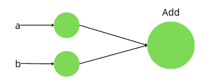
Let us add two variables using TensorFlow to understand how the graphs work. We have two variables, a=4 and b=5, and we want to add them. The tf.add() is a function in TensorFlow that is used to add variables. It has three arguments x, y, and name where x and y are the values to be added together and the name is the operation name as shown below:

# defining varriables
a = 4
b = 5
# addition using tensorflow
Sum = tf.add(a, b, name='Add')
# printing the sum
print(Sum)

Output:

As you can see, instead of getting just the value of the summation of the two variables, we get much more information. The addition code creates a graph with two input nodes and one output node for the addition operation (named Add). When we print out the variable Sum, it prints out the Tensor information; its name (Add), shape (() means scalar), and type (32-bit integer).

We didn’t get the answer 4 + 5 = 9 in the above code because the first step creates a graph, and to evaluate the nodes, we must run the graph within a Session. TensorFlow does not execute the graph unless it is specified to do so with a session. In simple words, the written code above only generates the graph, which determines the expected sizes of Tensors and operations to execute them. However, it doesn’t assign a numeric value to any Tensors. Hence, we need to create and run a session to assign these values and make them flow through the graph.

Now, let us create a Session and find the sum of the two variables.

# creating sessions in tensorflow
with tf.compat.v1.Session() as sess:
    # printing the sum with session
    print(sess.run(Sum))

Output:

Notice that this time we get the actual value of the summation.

Types of Tensor in TensorFlow

TensorFlow has its data structure for performance and ease of use. Tensor is the data structure used in Tensorflow (remember, TensorFlow is the flow of tensors in a graph). TensorFlow programs use a tensor data structure to represent all data, and only tensors are passed between operations in the computation graph. You can think of a TensorFlow tensor as an n-dimensional array or list.

Here we will go through some of the most used Tensor types.

Constant

In TensorFlow, the constants create nodes that take values which does not change. We can create a constant Tensor using tf.constant() function. Let us create constant values and add them.

# create constants in tensorflow
a = tf.constant(5)
b = tf.constant(4)
# Adding constants
Sun = a + b
# launch the graph in a session
with tf.compat.v1.Session() as sess:
    print(sess.run(Sum))

Output:

We can also define constants of different data types. For example, let us create a constant floating number and a matrix.

# Creating floating number
floating = tf.constant(5.3, name='scalar', dtype=tf.float32)
# creating matrix 
matrix = tf.constant([[1, 2], [3, 4]], name='matrix')
# launch the graph in a sessions
with tf.compat.v1.Session() as sess:
    print(sess.run(floating))
    print('\n')
    print(sess.run(matrix))

Output:

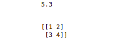
Notice that we had defined a floating number and a matrix.

Variable

Variables are nodes that output their current value. Unlike constants, their values can be changed over time. Let us create different data-typed variables with their initial values.

# create variable and initializing values
integer_value = tf.compat.v1.get_variable(name="var1", initializer=tf.constant(2))
floating_value = tf.compat.v1.get_variable(name="var2", initializer=tf.constant(3.54))
# add an Op to initialize global variable
init_op = tf.compat.v1.global_variables_initializer()
# launch the graph in a session
with tf.compat.v1.Session() as sess:
    
    # run the variable initializer operation
    sess.run(init_op)
    
    # printing valus of varibles
    print(sess.run(integer_value))
    print(sess.run(floating_value))

Output:

As you can see, we have used get_variable() function to create a variable.

Placeholder

Placeholders are more basic than a variable. It is simply a variable that we assign data in a future time. Placeholders are nodes whose value is fed in at execution time. If we have inputs to our network that depend on external data and don’t want our graph to depend on any real value while developing the graph, placeholders are the data type we need in such a case. For example, in the following code, we will define a placeholder first and add it with a constant, but we will assign the values to the placeholder while executing it.

# defining constand
cont = tf.constant([0, 0, 0], tf.float32, name='A')
# defining a place holder ( empty)
placeHolder = tf.compat.v1.placeholder(tf.float32, shape=[3], name='B')
# Adding constant and placeholder
Sum = tf.add(cont, placeHolder, name="Add")
with tf.compat.v1.Session() as sess:
    
    # create a dictionary assigning to placeholder
    d = {placeHolder: [1, 2, 3]}
    
    
    # feed it to the placeholder
    print(sess.run(Sum, feed_dict=d)) 

Output:

As you can see, we have initialized the values to the placeholder while executing it.

TensorBoard for visualizing Machine learning and Neural network models

As discussed earlier, all the numerical computations are expressed as a computational graph in TensorFlow. The TensorBoard helps us to visualize those computations graphically. Sometimes, the computations can be very complex and confusing. The TensorBoard helps us to debug, understand and visualize complex computations.

Visualizing the graph

Now let us see how we can set up and visualize the computations in TensorFlow using TensorBoard. We will first create two constants, add them, and then use TensorBoard to visualize the computations.

# To clear the defined variable and operations of the previous cell
tf.compat.v1.reset_default_graph()   
# create graph
a = tf.constant(10)
b = tf.constant(3)
c = tf.add(a, b)

# launch the graph in a session
with tf.compat.v1.Session() as sess:
    # or creating the writer inside the session
    writer = tf.compat.v1.summary.FileWriter('./graphs', sess.graph)

When we run this code, it creates a directory inside our current directory (besides the Jupyter notebook) which contains the events.

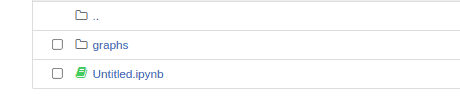
The next step is to go to the terminal or command line(make sure you open the terminal in the same directory where the Jupyter notebook is) and run the following commands.

tensorboard --logdir="./graphs" --port 6006

This will give us a link. Copy the link and paste it into any browser, and the TensorBoard will open.

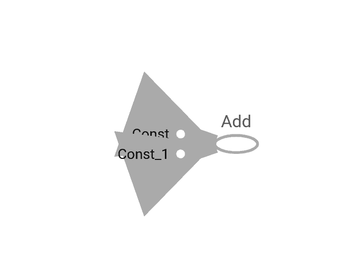
Here the const and const_1 represent the nodes for the constants, and the Add node represents the addition operation. Notice the names of the constants in the code are not the same as in the graph. The names of the nodes in the graph are assigned by default unless we explicitly define the names.

Now, let us explicitly define the names of the nodes in the graph.

# To clear the defined variables and operations of the previous cell
tf.compat.v1.reset_default_graph()   
# create graph
a = tf.constant(10,name="a")
b = tf.constant(3, name="b")
c = tf.add(a, b, name="addition")

# launch the graph in a session
with tf.compat.v1.Session() as sess:
    # or creating the writer inside the session
    writer = tf.compat.v1.summary.FileWriter('./graphs', sess.graph)

Now, the output graph in the Tensorboard looks like this:

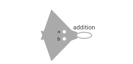
Notice that the names of nodes representing constants and the computation have been changed.

Let us make the graph more complicated by multiplying and adding the results.

# To clear the defined variables and operations of the previous cell
tf.compat.v1.reset_default_graph()   
# create graphs
a = tf.constant(10,name="a")
b = tf.constant(3, name="b")
c = tf.add(a, b, name="addition")
d = tf.math.multiply(c, a, name='multiplication')
f = tf.add(c, d, name='Final')
# launch the graphs in a session
with tf.compat.v1.Session() as sess:
    # or creating the writer inside the session
    writer = tf.compat.v1.summary.FileWriter('./graphs', sess.graph)

The graph will be:

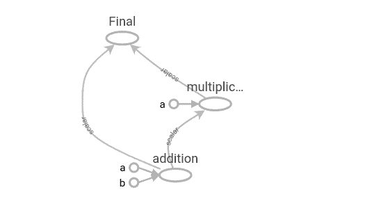
Notice that we first added two constants, multiplied the result with a constant a, and added the summation and multiplication results.

Visualizing the summaries

So far, we have only focused on how to visualize graphs in TensorBoard, but it has one more cool feature. In this section, we are now going to use a special operation called summary to visualize the model parameters (like weights and biases of a neural network), metrics (like loss or accuracy value), and images (like input images to a network). The summary is a special TensorBoard operation that takes in a regular tenor and outputs the summarized data.

There are three main types of TensorFlow graphs for summaries:

• summary.scalar: used to write a single scalar-valued tensor (like classification loss or accuracy value)
• summary.histogram: used to plot the histogram of all the values of a non-scalar tensor (like weight or bias matrices of a neural network).
• summary.image: Used to plot images (like input images of a network or generated output images of an autoencoder or a GAN).

In this section, we will explore the first two plots.

Let us first use summary.scalar() to summarize the information. It’s for writing a scalar-tensor’s values that change over time or iterations. A deep neural network (say, a simple network for classification tasks) is usually used to monitor the changes in loss function or classification accuracy. Here we will take 100 random values from the Normal distribution and then plot them using summary.scalar().

# To clear the defined variables and operations of the previous cell
tf.compat.v1.reset_default_graph()   
# create the scalar variable from normal distribution
x_scalar = tf.compat.v1.get_variable('x_scalar', shape=[], initializer=tf.compat.v1.truncated_normal_initializer(mean=0, stddev=1))
# create the scalar summary
first_summary = tf.compat.v1.summary.scalar(name='Summary_of_random_variables', tensor=x_scalar)
# initializing the global variable
init = tf.compat.v1.global_variables_initializer()
# launch the graphs in a session
with tf.compat.v1.Session() as sess:
    
    # creating the writer inside the session
    writer = tf.compat.v1.summary.FileWriter('./graphs', sess.graph)
    # model iteration
    for step in range(100):
        
        # loop over several initializations of the variable
        sess.run(init)
        
        # evaluate the scalar summary
        summary = sess.run(first_summary)
        
        #add the summary to the writer
        writer.add_summary(summary, step)

Once you run the above program and refresh the TensorBoard, you will see a new tab named ‘Scalars” click on it to see the summary.scalar plots. The above code will produce the following graph.

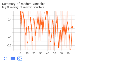
The x-axis and y-axis show the 100 steps and the corresponding values of the variable, respectively.

Now we will use summary.histogram(), which is used to plot the histogram of the values of a non-scalar tensor. This gives us a view of how the histogram/distribution of the tensor values change over time or iterations. In the case of neural networks, it’s commonly used to monitor the changes in weights and biases distributions.

We will use the same example ( random numbers from a normal distribution) to plot a histogram. Here we will add a matrix of size 40X40 whose entries come from a standard normal distribution. In the example, we will initialize this matrix 100 times and plot the distribution of its entries over time using summary.histogram().

 # To clear the defined variables and operations of the previous cell
tf.compat.v1.reset_default_graph()  
# create the variables in tensorflow code
x_matrix = tf.compat.v1.get_variable('x_matrix', shape=[40, 40], initializer=tf.compat.v1.truncated_normal_initializer(mean=0, stddev=1))
# A histogram summary/model distribution for the non-scalar tensor
histogram_summary = tf.compat.v1.summary.histogram('histogram_summary', x_matrix)
#initializing input data/variables
init = tf.compat.v1.global_variables_initializer()
# launch the graphs in a session
with tf.compat.v1.Session() as sess:
    
    # creating the writer inside the session
    writer = tf.compat.v1.summary.FileWriter('./graphs', sess.graph)
    # model iteration
    for step in range(100):
        # loop over several initializations of the variable
        sess.run(init)
        # evaluate the merged summaries/ model distribution
        summary = sess.run(histogram_summary)
        
        # the histogram summary
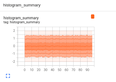
        writer.add_summary(summary, step)

After running the above code, when you refresh the TensorBoard, new tabs have been added ( Distribution and Histogram). Click on them to see the following Outputs:

Plot under ‘Distribution”:

And the plot under ‘Histogram” is:

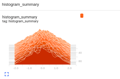
As you see in the figure, the “Distributions” tab contains a plot showing the tensor values distribution. Each line on the chart represents a percentile in the data distribution. These percentiles can also be considered standard deviation boundaries on a normal distribution. Similarly, in the histogram panel, each chart shows temporal “slices” of data, where each slice is a histogram of the tensor at a given step. One more cool feature of these plots is that they are interactive. We can move the cursor over them and see x and y values.

Building ANN in TensorFlow

Now that we have basic knowledge of TensorFlow and Neural networks, we will build a simple ANN on the Fashion MNIST dataset, which consists of 70,000 images, out of which 60,000 images belong to the training and 10,000 images belong to the test set. Each image is 28 pixels in height and 28 pixels in width. The dataset contains information about the following images:

• T-Shirt ( represented by 0)

• Trouser ( represented by 1)

• Pullover ( represented by 2)

• Dress( represented by 3)

• Coat ( represented by 4)

• Sandal ( represented by 5)

• Shirt ( represented by 6)

• Sneaker ( represented by 7)

• Bag ( represented by 8)

• Ankle Boot ( represented by 9)

Importing Dataset

Now let us import the dataset. The dataset is in the submodule of TensorFlow datasets, so we have to import it from there.

# load data
from tensorflow.keras.datasets import fashion_mnist
# loading the testing and training dataset
(X_train, y_train), (X_test, y_test) = fashion_mnist.load_data()

As we know that images are stored in the form of matrices. If we print out any loaded data, we see that they are just matrices.

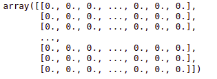
#Training dataset /multidimensional data arrays
X_train

Output:

Now let us print out the output class as well.

#Output class
y_train

Output:

As you can see, the output values are from 0 to 9, which represent different images.

We will normalize the data so that the ANN model will train faster. We will divide each image by the maximum number of pixels(255) so that the image range will be between 0 and 1.

# Normalizing the dataset
X_train = X_train/255.0
X_test = X_test/255.0

The next step is to reshape the dataset.

# Reshaping the dataset /matrix multiplication
X_train = X_train.reshape(-1, 28*28)
X_test = X_test.reshape(-1, 28*28)

Now the dataset is ready, so we will move to build the ANN model

Building Deep learning models using TensorFlow

The first step of building an ANN model using TensorFlow is creating a model object.

# Creating a model object
model = tf.keras.models.Sequential()

Now, we will make the first fully connected layer of the ANN. It takes the following parameters.

• Number of neurons (in our case, 128)
• Activation function (We will use ReLU)
• input shape (784, )

We add all these hyperparameters using the model.add() method.

# Frist fully connected input layer
model.add(tf.keras.layers.Dense(units = 128, activation = 'relu', input_shape = (784,)))

Now, we will add a dropout layer. Dropout is simply a regularization technique where we randomly set neurons in a layer to zero. In this way, some percentage of neurons won’t be updated. The training process is long, and we have less chance of overfitting.

# Adding drop out layer to learning models
model.add(tf.keras.layers.Dropout(0.2))

For simplicity, we will not create any hidden layer. So, the last part of the building NN is adding an output layer. The two most important parameters of the output layer are:

• units: It represents the number of classes (In our case, there are 10 )
• activation: We will use the softmax function.

# Output Layers #softmax for multi classsification and sigmoid for binary classification
model.add(tf.keras.layers.Dense(units = 10, activation = 'softmax'))

As soon as we have built the ANN, we must compile it. Compiling the model means connecting the whole network to an optimizer and choosing a loss. An optimizer is a tool that will update the weights during stochastic gradient descent.

# compiling the learning models 
model.compile(optimizer = 'adam', loss = 'sparse_categorical_crossentropy', metrics = ['sparse_categorical_accuracy'])

Training and testing the model

Now that our ANN is ready, we will train it on the Training dataset.

# tensorflow run model/train model
model.fit(X_train, y_train, epochs =5)

Once the training is done, we can then use the testing data to test and predict the output categories and evaluate the model to see how well our model performs.

# predict and Evaluating the model
test_accuracy = model.evaluate(X_test, y_test)

Let us now print the accuracy score.

# accuracy score
print(test_accuracy)

Output:

This shows that our model could accurately classify 87% of the testing data.

Summary

TensorFlow is a powerful Machine learning and neural network library that help us to build models, which Google researchers initially developed. It contains many built-in APIs for the implementation of various neural network algorithms. You can implement it on multiple platforms, including websites (Tensoflow.js ), Mobile, and Edge(TensorFlow lite). In this tutorial, we learned the basics of TensorFlow, from its installation to its implementation. We discussed TensorFlow’s applications and some essential features. Moreover, we built a deep learning model, trained it, and tested the model as well.

For more in-depth information about Tensorflow, we strongly recommend you check out one of the most popular Udemy courses – Python for Data Science and Machine Learning Bootcamp.