Linear Discriminant Analysis in Machine Learning: A Beginner’s Guide
Linear Discriminant Analysis (LDA), also known as Normal Discriminant Analysis or Discriminant Function Analysis, is a dimensionality reduction technique commonly used for projecting the features of a higher dimension space into a lower dimension space and solving supervised classification problems. In this article, we will cover Linear Discriminant Analysis in-depth and demonstrate how you can use it to reduce the dimensions of datasets using Python. We will use Amazon SageMaker and Jupyter notebooks for implementation and visualization purposes.
Table of contents
Before going into the Linear Discriminant Analysis, it is highly recommended to go through the Principal Component Analysis (PCA) algorithm because there are many similarities between PCA and LDA.
Explanation of Linear Discriminant Analysis
Linear Discriminant Analysis is used for classification, dimension reduction, and data visualization. But its main purpose is dimensionality reduction. Despite the similarities to Principal Component Analysis (PCA), LDA differs in one crucial aspect. Instead of finding new axes (dimensions) that maximize the variation in the data, it focuses on maximizing the separability among known categories (classes).
Another feature that differentiates the LDA from PCA is that the Linear Discriminant Analysis falls under the Supervised Machine Learning algorithms category. That means you must have the output class examples in your dataset to educate your model.
We can easily visualize and analyze the data if we have a dataset in one dimension, two-dimension, or even three dimensions. But things become more complex when we have datasets of more than three dimensions. It becomes difficult to visualize such a dataset. In such cases, Linear Discriminant Analysis helps us to reduce dimensions and visualize the dataset using three or two dimensions.
Let’s take a very simple two-dimensional dataset and apply the LDA to reduce it to the one-dimensional dataset.
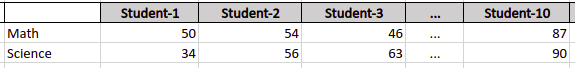
Out simple dataset contains the obtained marks of 10 students in Math and Science subjects. Let’s say the following picture is the visualization of the dataset.
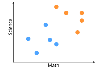
Let’s assume that the blue dots show the students who got less than 70% in both subjects, and the orange dots represent the students who got above 70%. Now, we can apply the LDA to reduce the data to one dimension without losing the information.
LDA uses both the axes (Math and Science) to create a new axis. Then it projects the data onto this new axis to maximize the separation of the two categories.
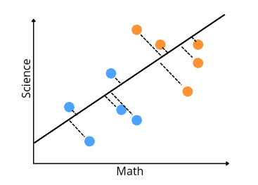
This new axis is created according to two criteria that are considered simultaneously:
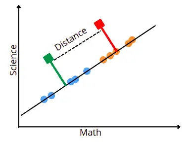
- The first criterion is to maximize the distance between means of data values. In our case, the distance between means of low-scoring and high-scoring students.
- The new axis’s second criterion is minimizing the variance within each category. The variance in LDA is called scatter and is represented by an S2.
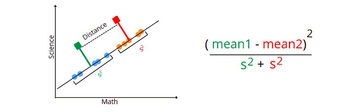
The LDA uses the above equation to find the optimum axis to project the dataset on the newly created axis and consider it a dimension for the dataset.
Once the algorithm finds the optimum axis, it projects the dataset onto it and considers this axis as a new axis for the dataset. For example, in our case, the data dimensionality is reduced to one dimension, as shown below:

Similarly, if the dataset is three-dimensional, then two new axes will be created to reduce data dimensions.
Implementation of LDA
Let’s implement the LDA on the Iris dataset. This dataset contains information about the size of the petals and sepals of three different species of flowers.
Before implementing the LDA on the given dataset, ensure you have installed the following modules on your system.
- pandas
- NumPy
- matplotlib
- sklearn
- seaborn
You can install the required modules by running the following commands in the cell of Jupyter Notebook.
%pip install pandas
pip install numpy
pip install matplotlib
pip install sklearn
pip install seaborn
Once the installation is complete, we are good to go.
Importing and exploring the dataset
The Iris dataset is available in the submodule of the sklearn module, so we can directly load the data from there and explore it.
# importing the module
from sklearn import datasets
# loading the iris data
dataset  = datasets.load_iris()
Let’s print the keys of the dataset and see what kind of information we have there:
# dataset key values
dataset.keys()
Output:

You can explore each of these on your own, but here we will just go through DESCR because it contains the details about the dataset.
# information about dataset
print(dataset['DESCR'])
Output:
Iris plants dataset
--------------------
**Data Set Characteristics:**
    :Number of Instances: 150 (50 in each of three classes)
    :Number of Attributes: 4 numeric, predictive attributes and the class
    :Attribute Information:
        - sepal length in cm
        - sepal width in cm
        - petal length in cm
        - petal width in cm
        - class:
                - Iris-Setosa
                - Iris-Versicolour
                - Iris-Virginica

    :Summary Statistics:
    ============== ==== ==== ======= ===== ====================
                    Min  Max   Mean    SD   Class Correlation
    ============== ==== ==== ======= ===== ====================
    sepal length:   4.3  7.9   5.84   0.83    0.7826
    sepal width:    2.0  4.4   3.05   0.43   -0.4194
    petal length:   1.0  6.9   3.76   1.76    0.9490  (high!)
    petal width:    0.1  2.5   1.20   0.76    0.9565  (high!)
    ============== ==== ==== ======= ===== ====================
    :Missing Attribute Values: None
    :Class Distribution: 33.3% for each of 3 classes.
    :Creator: R.A. Fisher
    :Donor: Michael Marshall (MARSHALL%PLU@io.arc.nasa.gov)
    :Date: July, 1988
The famous Iris database, first used by Sir R.A. Fisher. The dataset is taken
from Fisher's paper. Note that it's the same as in R, but not as in the UCI
Machine Learning Repository, which has two wrong data points.
This is perhaps the best known database to be found in the
pattern recognition literature.  Fisher's paper is a classic in the field and
is referenced frequently to this day.  (See Duda & Hart, for example.)  The
data set contains 3 classes of 50 instances each, where each class refers to a
type of iris plant.  One class is linearly separable from the other 2; the
latter are NOT linearly separable from each other.
.. topic:: References
   - Fisher, R.A. "The use of multiple measurements in taxonomic problems"
     Annual Eugenics, 7, Part II, 179-188 (1936); also in "Contributions to
     Mathematical Statistics" (John Wiley, NY, 1950).
   - Duda, R.O., & Hart, P.E. (1973) Pattern Classification and Scene Analysis.
     (Q327.D83) John Wiley & Sons.  ISBN 0-471-22361-1.  See page 218.
   - Dasarathy, B.V. (1980) "Nosing Around the Neighborhood: A New System
     Structure and Classification Rule for Recognition in Partially Exposed
     Environments".  IEEE Transactions on Pattern Analysis and Machine
     Intelligence, Vol. PAMI-2, No. 1, 67-71.
   - Gates, G.W. (1972) "The Reduced Nearest Neighbor Rule".  IEEE Transactions
     on Information Theory, May 1972, 431-433.
   - See also: 1988 MLC Proceedings, 54-64.  Cheeseman et al"s AUTOCLASS II
     conceptual clustering system finds 3 classes in the data.
   - Many, many more ...
Next, you can find the dataset’s statistics by using the Pandas DataFrame describe() function.
# importing the module
import pandas as pd
# convertig the dataset into pandas dataframe
data = pd.DataFrame(dataset.data, columns=dataset.feature_names)
# descriptive statistics
data.describe()
Output:
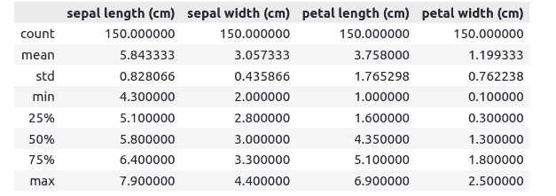
DataFrame’s stats contain each column’s count, such as mean, standard deviation, minimum, maximum values, etc.
Using LDA for dimensionality reduction
There are 4 input variables in our dataset, so it is impossible to visualize them in one graph. Let’s apply LDA with 2 components so that the same data can be visualized using the 2D plot.
# input and output variables
X = dataset.data
y = dataset.target
target_names = dataset.target_names
# importing the requried module
from sklearn.discriminant_analysis import LinearDiscriminantAnalysis
# initializing the model with 2 components
lda = LinearDiscriminantAnalysis(n_components=2)
# fitting the dataset
X_r2 = lda.fit(X, y).transform(X)
Now our data is two-dimensional, and we can easily visualize it.
# importing the required module
import matplotlib.pyplot as plt
# plot size
plt.figure(figsize=(15, 8))
# plotting the graph
plt.scatter(X_r2[:,0],X_r2[:,1],  c=dataset.target)
plt.show()
Output:
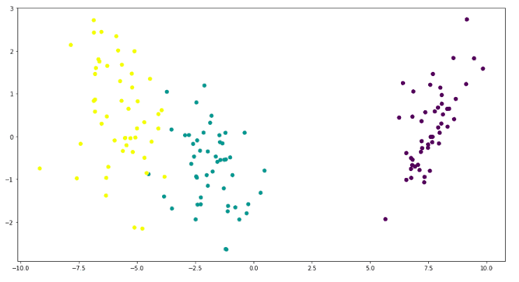
This graph shows that there are three types of output classes. The LDA has helped us to visualize these three clusters in a 2D plot.
Visualization of LDA components
Now let’s visualize the distribution of the dataset for each component using the Box plot.
# importing the required module
import seaborn as sns
# creating the dataframe
df=pd.DataFrame(zip(X_r2[:,0],X_r2[:,1],y),columns=["ld1","ld2","class"])
# setting the size of the image
sns.set(rc={'figure.figsize':(12,8)})
# plotting the graphs
subplot(2,1,1)
sns.boxplot(x='class', y='ld1', data=df)
subplot(2,1,2)
sns.boxplot(x='class', y='ld2', data=df)
Output:
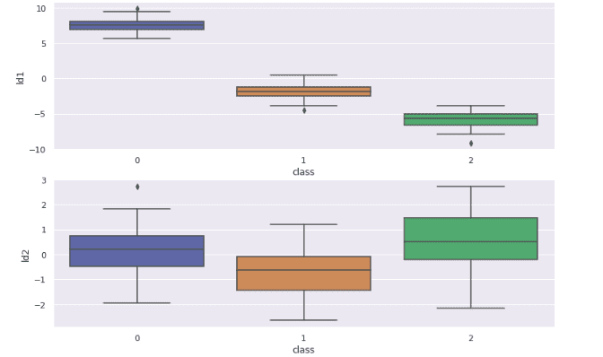
The above plot shows how the LDA has distributed the dataset based on their target variables in different components. We can also see that some classes contain outliers.
LDA vs PCA (visualization differences)
Now, let’s apply the PCA on the same dataset to reduce it to 2 dimensions as we did with the help of LDA and compare the results.
First, let’s fit the PCA model on the training dataset:
# importing the required moduel
from sklearn.decomposition import PCA
# PCA with 2 components
pca = PCA(n_components=2)
X_pca = pca.fit(X).transform(X)
Once the training is complete, we can visualize clusters:
# importing the module
from pylab import *
# subploting and title setting
subplot(2,1,1)
title("PCA")
# plotting the pca
plt.scatter(X_pca[:,0],X_pca[:,1], c=dataset.target)
# subploting and title
subplot(2,1,2)
title("LDA")
# plotting LDA
plt.scatter(X_r2[:,0],X_r2[:,1], c=dataset.target)
plt.show()
Output:
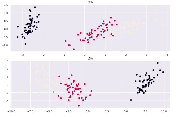
Both algorithms have successfully reduced the components but created different clusters because both have reduced the components based on different principles.
Now let’s also visualize and compare the distributions of each of the algorithms on their respective components. Here we will visualize the distribution of the first component of each algorithm (LDA-1 and PCA-1).
# creating dataframs
df=pd.DataFrame(zip(X_pca[:,0],X_r2[:,0],y),columns=["pc1","ld1","class"])
# plotting the lda1
subplot(2,1,1)
sns.boxplot(x='class', y='ld1', data=df)
# plotting pca1
subplot(2,1,2)
sns.boxplot(x='class', y='pc1', data=df)
Output:
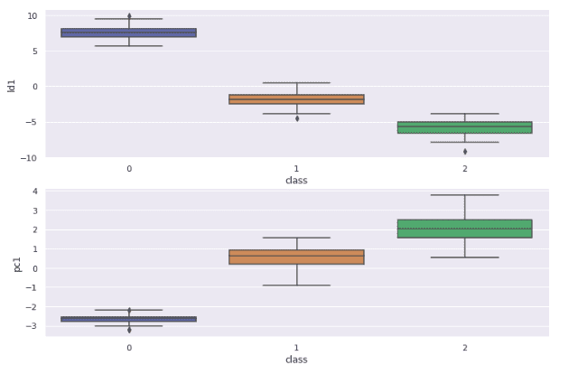
There is a slight difference in the distribution of both of the algorithms. For example, the PCA result shows outliers only at the first target variable, whereas the LDA result contains outliers for every target variable.
Using LDA to solve a classification problem
The Linear Discriminant Analysis algorithm can be used as a classifier for categorical variables. Let’s take a look at how to do it.
First, let’s split the dataset into testing and training parts.
# importing the module
from sklearn.model_selection import train_test_split
# splitting the dataset
X_train, X_test, y_train, y_test = train_test_split(X, y, test_size=0.25)
We assigned 25% of the data to the testing and the remaining 75% to the training.
Now, we can initialize the model and train it:
# initializing the model
lda_model = LinearDiscriminantAnalysis(n_components=2)
# training the model
lda_model.fit(X_train, y_train)
Once the training is complete, we can go to the testing part:
# testing the model
y_pred = lda_model.predict(X_test)
Let’s evaluate the model using an accuracy score:
# importing required module
from sklearn.metrics import accuracy_score
# printing the accuracy
print(accuracy_score(y_test, y_pred))
Output:
This shows that the LDA classifier correctly classified 97% of the testing data.
Summary
Linear Discriminant Analysis (LDA) or Discriminant Function Analysis is a dimensionality reduction technique commonly used to project the features of a higher dimension space into a lower dimension space and solve supervised classification problems. In this article, we’ve covered the Linear Discriminant Analysis algorithm and demonstrated how to use it to reduce the dimensions of datasets using Python.
