Isolation Forest For Anomalies Detection
Anomaly detection identifies data points in data that don’t fit the normal patterns. It can be useful to solve many problems, including fraud detection, medical diagnosis, etc. Machine Learning algorithms can help automate anomaly detection and make it more effective, especially when large datasets are involved. One of the methods to detect anomalies in a dataset is the Isolation Forest algorithm. This article will cover the Isolation Forest algorithm, how it is working, and how to apply it to various kinds of datasets.
Table of contents
Before starting with the Isolation Forest, make sure that you are already familiar with the basic concepts of Random Forest and Decision Trees algorithms because the Isolation Forest is based on these two concepts.
Explanation of Isolation Forest algorithm
Isolation Forest is an Unsupervised Machine Learning algorithm that identifies anomalies by isolating outliers in the data. An outlier is nothing but a data point that differs significantly from other data points in the given dataset.
Isolation Forest is based on the Decision Tree algorithm and it isolates the outliers by randomly selecting a feature from the given set and randomly selecting a split value between the max and min values. Such random features partitioning produces shorter paths in trees for the anomalous data points, thus distinguishing them from the rest of the data.
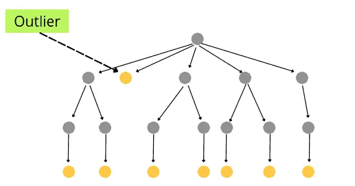
When the decision tree is created, it takes fewer nodes to reach the outliers than other normal data points.
The good thing about the Isolation Forest algorithm is that it can directly detect anomalies using isolation (how far a data point is from the rest of the data). The algorithm can run in a linear time complexity like other distance-related models such as K-Nearest Neighbors. The Isolation Forest detects anomalies by introducing binary trees that recursively generate partitions by randomly selecting a feature and then randomly selecting a split value for the feature. The partitioning process will continue until it separates all the data points from the rest of the samples.
Let’s take a sample dataset to understand how the Isolation Forest algorithm detects an outlier. Let’s say we have the following data point:
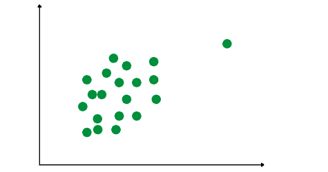
The algorithm will start building binary decision trees by randomly splitting the dataset. Let’s assume it splits the data in the following way:
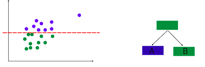
After that, the algorithm will split the data randomly and continue building the decision tree. Let’s assume this time the split looks like this:

The same process of a random split will continue until all the data points are separated.
Let’s assume that the algorithm was able to isolate one of the data points this time:
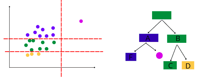
The algorithm takes three splits to isolate the above point. At the same time, if the algorithm continues the splitting process, it will take more time to isolate other points because they are close to each other (way more iterations will be required).
The algorithm will create a random forest of such decision trees and calculate the average number of splits to isolate each data point. The lower number of split operations needed to isolate a point, the more chance the data point will be an outlier.
After isolating all the data points, the algorithm uses the following equation to detect anomalies:
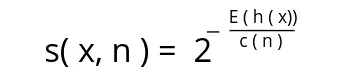
In the above equation:
- n – is the number of external nodes
- h(x) – is the path length of observation
x - c(n) – is the average path length of an unsuccessful search in a binary tree
So, the above equation will give each observation an anomaly score. If the anomaly score is close to 1, the point is considered to be an outlier. If the score is smaller than 0.5, then observation is considered to be normal. If all the scores are close to 0.5, the entire dataset does not have clear anomalies.
Applying Isolation Forest to regression dataset
A dataset having continuous output values is known as a regression dataset. Here we will take the house price dataset and detect if our dataset contains any outlier based on the prices of the houses.
Before going to the implementation part, ensure that you have installed the following Python modules on your system:
- numpy
- pandas
- seaborn
- sklearn
- plotly
You can install the above-required modules by running the following commands in the cell of the Jupyter notebook.
%pip install numpy
%pip install pandas
%pip install seaborn
%pip install sklearn
%pip install plolty
Once the installation is complete, we can then start the implementation part.
Importing and exploring the dataset
We will use Pandas DataFrame to work with the dataset and explore it.
# importing the pandas
import pandas as pd
# importing the dataset
dataset = pd.read_csv('Dushanbe_house.csv')
# printing the head
dataset.head()
Output:
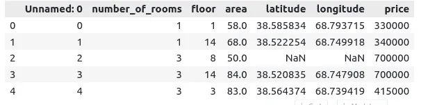
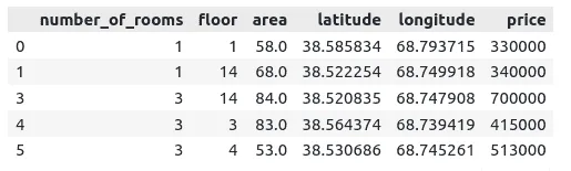
Notice that our dataset contains some NULL values and an unnecessary column of index values. Let’s remove them from the dataset:
# removing the indexed column
dataset.drop('Unnamed: 0', axis=1, inplace=True)
# removing null values
dataset.dropna(inplace=True)
# heading
dataset.head()
Output:
Let’s plot the dataset to see if we have any outliers or not:
# importing the module
import plotly.express as px
# plotting scattered graph
fig = px.scatter([i for i in range(len(dataset['price']))], y=dataset['price'])
fig.show()
Output:
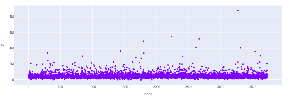
The visualization shows that there are some anomalies in the dataset. Let’s apply the Isolation Forest algorithm to detect them.
Training Isolation Forest model
Let’s train the Isolation Forest model using our dataset. Pay attention, that we will not split the dataset into the testing and training parts as the Isolation Forest belongs to Unsupervised Machine Learning algorithms.
# importing the required module
from sklearn.ensemble import IsolationForest
# initializing the isolation forest
isolation_model = IsolationForest(contamination = 0.003)
# training the model
isolation_model.fit(dataset)
# making predictions
IF_predictions = isolation_model.predict(dataset)
The contamination parameter defines a rough estimate of the percentage of the outliers in our dataset. So, we have assigned contamination to be 0.3% in our case.
Let’s print the predictions of the model:
# printing
print(IF_predictions)
Output:
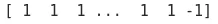
Notice that all the predictions are either 1 or -1. Where 1 shows the data point is normal while -1 represents the outliers.
Let’s plot the outlier using a different color on the same scattered plot:
# adding the anomalies to the dataset
dataset['anomalies'] = IF_predictions
anomalies = dataset.query('anomalies == -1')
# importing the plot
import plotly.graph_objects as go
# plotting the graph for outliers
normal = go.Scatter(x=dataset.index.astype(str),y=dataset['price'],name="Dataset",mode='markers')
outlier = go.Scatter(x=anomalies.index.astype(str),y=anomalies['price'],name="Anomalies",mode='markers',
                marker=dict(color='red', size=6,
                            line=dict(color='red', width=1)))
# labeling the graph
layout = go.Layout(title="Isolation Forest",yaxis_title='Price',xaxis_title='x-axis',)
# plotting
data = [normal, outlier]
fig = go.Figure(data=data, layout=layout)
fig.show()
Output:
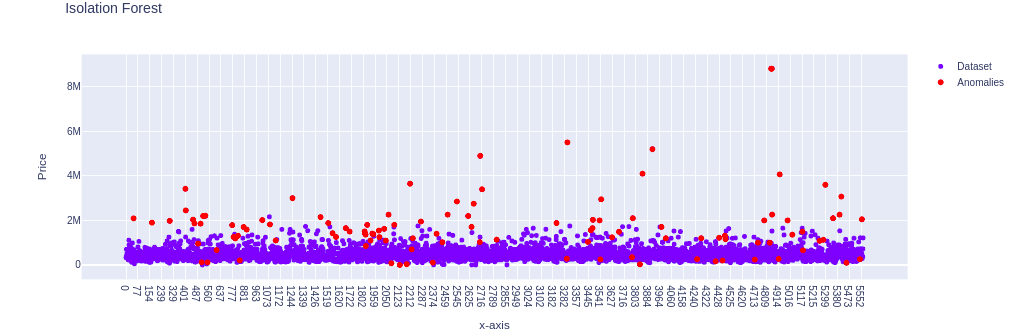
By looking at the above plot, you might be wondering why some of the data points have been incorrectly classified as anomalies by the algorithm as some of the red dots seem to be not outliers. However, that is not true. The algorithm has classified the above (red) points as anomalies based on all input variables. We’re visualizing only the price column, so don’t be confused with the obtained result. Some points may not be anomalies based on the price data only, but other parameters of the same data points allow us to treat them as anomalies.
Let’s remove some columns and try to detect the anomalies, to see how the input variables affect the detection process.
Training Isolation Forest model (reduced set of features)
Let’s remove the area, the number of floors, and the number of rooms variables and train the model using only location and price information.
# copying the dataset
data = dataset.copy()
# droping columns
data.drop('anomalies', axis=1, inplace=True)
data.drop('number_of_rooms', axis=1, inplace=True)
data.drop('area', axis=1, inplace=True)
data.drop('floor', axis=1, inplace=True)
# printing the head
data.head()
Now we can train the model using the same contamination parameter value (0.3%).
# initializing the isolation forest
isolation_model1= IsolationForest(contamination=0.003)
# training the model
isolation_model1.fit(data)
# making predictions
IF_predictions1 = isolation_model1.predict(data)
Now let’s plot the outlier detected by the model again:
# adding the anomalies to the dataset
data['anomalies'] = IF_predictions1
anomalies1 = data.query('anomalies == -1')
# plotting the scattered plot
normal = go.Scatter(x=data.index.astype(str),y=data['price'],name="Normal data", mode='markers')
outlier = go.Scatter(x=anomalies1.index.astype(str), y=anomalies1['price'], name="Anomalies", mode='markers',
                        marker=dict(color='red', size=5,
                            line=dict(color='red', width=1)))
# labelling
layout = go.Layout(title="Isolation Forest", yaxis_title='price',xaxis_title='x-axis',)

# plotting
Data = [normal, outlier]
fig = go.Figure(data=Data, layout=layout)
fig.show()
Output:
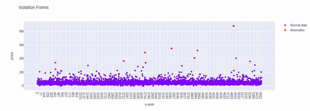
Pay attention that anomalies have been caught up by the algorithm this time because we trained the model based on the reduced feature set (location and prices data).
You can play with it by training the model on each of the columns separately and then visualizing the anomalies as we did here.
Applying Isolation Forest to classification dataset
A dataset that contains categorical values as output is known as a classification dataset. In this section, we will use a dataset about credit card transactions. The dataset contains transactions made by credit cards in September 2013 by European cardholders. This dataset presents transactions that occurred in two days, where we have 492 frauds out of 284,807 transactions. The dataset is highly unbalanced because the positive class (frauds) account for 0.172% of all transactions. Let’s use the Isolation Forest algorithm to detect fraud transactions and calculate how accurately the model predicts them.
Importing and exploring the dataset
First, let’s import the dataset and print out the few rows to get familiar with the data type.
# importing the dataset
credit_card = pd.read_csv("creditcard.csv")
# heading
credit_card.head()
Output:

Notice that the dataset contains 30 different columns storing transactions data, and the last column is the output class. Columns V1, V2, V3, …, and V28 are a result of the PCA transformation. According to the official dataset website (OpenML), features V1, V2, …, and V28 are the principal components obtained by PCA, and the only features which have not been transformed with PCA are ‘Time’ and ‘Amount.’
Let’s plot the output category using a bar chart:
# importing the module
import seaborn as sns
# setting the size of plotting
sns.set(rc={'figure.figsize':(15,8)})
# plotting bar plot
sns.countplot(credit_card['Class'])
Output:
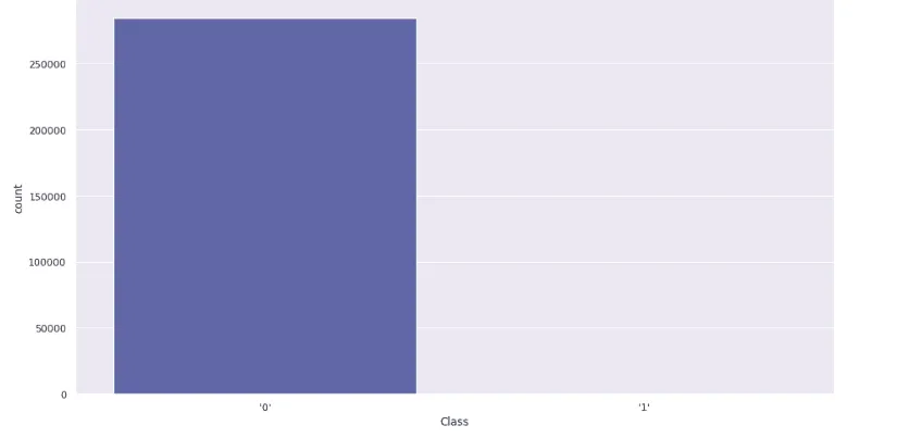
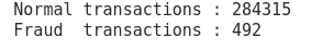
Notice that the fraud category is extremely lower compared to the normal transactions. Let’s print out the total number of fraud and normal transactions:
# stroing the normal and fraud cases
fraud = credit_card[credit_card['Class']=="'1'"]
valid = credit_card[credit_card['Class']=="'0'"]
# printing
print("Normal transactions :", len(valid))
print("Fraud  transactions :", len(fraud))
Output:
Let’s now use the info() method to get information about the data type in each column:
# info method
credit_card.info()
Output:
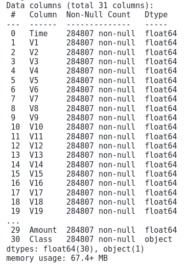
Notice that except for the output class, every column has numeric data. So, before training the model, we need to change the last column to numeric values too.
# Import label encoder
from sklearn import preprocessing

# label_encoder object knows how to understand word labels.
label_encoder = preprocessing.LabelEncoder()

# Encode labels in column 'species'.
credit_card['Class']= label_encoder.fit_transform(credit_card['Class'])
Now, our data is ready to be used by the Isolation Forest algorithm.
Training and testing the Isolation forest model
We can split the dataset into testing and training parts to evaluate the Isolation Forest once it detects the outliers because we know upfront that the fraud category represents outliers. After that, we will compare the actual fraud cases and the model predicted outliers.
# splitting the dataset into input and outputs
columns = credit_card.columns.tolist()
columns = [c for c in columns if c not in ['Class']]
X = credit_card[columns]
Y = credit_card['Class']
# importing the module
from sklearn.model_selection import train_test_split
# splitting the dataset
X_train,X_test,Y_train,Y_test = train_test_split(X,Y,test_size = .20)
Now let’s use the training data to train the model.
# initializing the model
clf = IsolationForest(max_samples=len(X_train))
# training the model
clf.fit(X_train)
We have applied only the input data to train the model because it is an Unsupervised Learning algorithm. Once training is complete, we can make predictions:
# making predictions
y_pred = clf.predict(X_test)
We already know that the predicted values of the Isolation forest will be -1 and 1. Where -1 represents the outlier and 1 represents the normal value. 0 represents the normal value in the actual dataset, and 1 represents the fraud so we will change the predictions to 0 and 1.
# changing the predicted values
y_pred[y_pred==1] = 0
y_pred[y_pred==-1] = 1
Let’s find the accuracy of the Isolation Forest by using its predicted and the actual values:
# importing the module
from sklearn.metrics import accuracy_score
# finding the accuracy
print(accuracy_score(y_pred,Y_test))
Output:
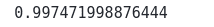
The result shows that the model has classified fraud and valid transactions in 99.7% of cases.
If you want to know how we can apply the Isolation forest to the Time series, look at the Implementing anomaly detection using Python article.
Summary
The Isolation Forest is an Unsupervised Machine Learning algorithm that detects the outliers in a dataset by building a random forest of decision trees. In this article, we’ve covered the Isolation Forest algorithm, its logic, and how to apply it to solve regression and classification problems.
