Using the Random Sample Consensus (RANSAC) algorithm in Python

RANdom SAmple Consensus (RANSAC) is a Supervised Machine Learning iterative outlier detection algorithm. Unlike the Linear Regression algorithm which predictions are highly affected by the outlier, the RANSAC algorithm creates the best-fitted line/predictions based on only inliers, not outliers. This article will cover how the RANSAC algorithm works, show how the predicted line of RANSAC differs from the Linear Regression, and apply the RANSAC algorithm to solve the regression problem. We will use Amazon SageMaker Studio and Jupyter notebooks for implementation and visualization.

Before starting the RANSAC algorithm, make sure that you understand the Linear Regression algorithm and its various evaluation scores. By default, the modeling method in RANSAC is linear regression.

Explanation of the RANSAC algorithm

The RANSAC stands for RANdom SAmple Consensus – a regression algorithm that trains the model by handling the outliers. An outlier is a data point that is noticeably different from the rest. They represent measurement errors, bad data collection, or show variables not considered when collecting the data. Most Machine Learning algorithms are highly affected by outliers in the dataset because they are influencing algorithms’ predictions.

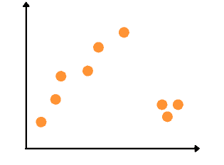
For example, let’s take the following sample of data points:

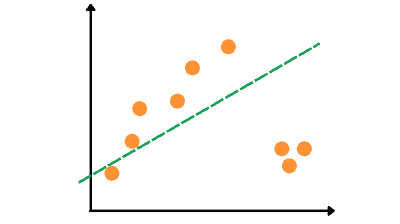
The Linear Regression algorithm will give us a predicted best-fitted line highly affected by the outliers:

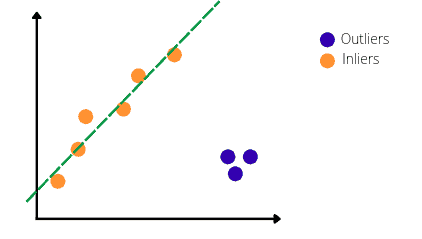
The RANSAC algorithm will identify the outliers in the dataset and train the model only on the inliers. So, the best-fitted line produced by RANSAC algorithm will be:

Let’s take a look at how the RANSAC algorithm finds the best-fitted line and ignores the outliers.

Keep in mind that the RANSAC algorithm is a repetitive algorithm that follows the same process repeatedly until it completes all iterations or finds the best result. For simplicity, let’s assume that the maximum number of iterations is 3.

The first step of the algorithm is to take any two random data points from the whole dataset and find the line passing through those points. The reason why it takes two points is that our dataset is two-dimensional. In the case of the three-dimensional dataset, the algorithm will take three random data points.

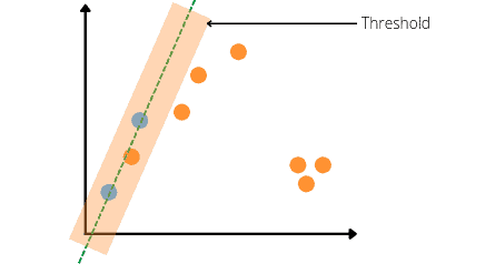
Let’s assume that it selects the following two points and finds the line that passes through them, as shown below:

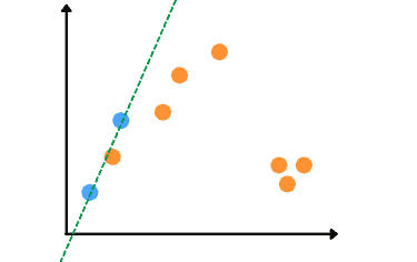
Now, the algorithm classifies and counts outliers and inliers data points based on a threshold value. Any dataset that falls within the threshold range will be considered as inliers. For example, see the visualization below that contains 3 inliers:

Now the algorithm completes the first iteration and gets the predicted line along with inliers and outliers. If we had a total number of iterations equal to 1, then the above line would be the predicted line of the algorithm, but in our example, we need two more iterations. So, the algorithm will continue the iterations by selecting two random data points again.

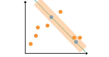
Let’s assume this time the algorithm selects the following two points and finds the line that passes through them (3 inliers):

The exact process will repeat the third (last) time, and the algorithm will select another two random data points and identify outliers and inliers based on the threshold value. Let’s assume, that this time the algorithm selected the following two points and got the following results (6 inliers).

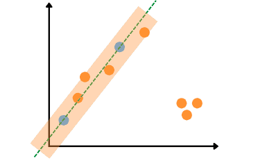
As soon as the algorithm completed the maximum number of iterations, it will select the results of the iteration with a maximum number of inliers – the last iteration in our example:

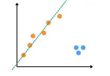
Finally, the algorithm will make the predictions for the testing data based on the obtained best-fitted line independent of the outliers in the dataset.

Applying the RANSAC algorithm to the regression dataset

Let’s apply the RANSAC algorithm to a regression dataset. We will use a dataset containing houses prices in Dushanbe city. The input variables are the area, location, number of floors, and rooms. You can download the dataset from this link.

Before going to the implementation part, ensure that you have installed the following modules as we will be using them.

• sklearn
• numpy
• pandas
• matplotlib

You can install them on your system by running the following commands in the cell of the Jupyter notebook.

%pip install sklearn
%pip install numpy
%pip install pandas
%pip install matplotlib

Once the installation is complete, we can start the coding part.

Importing the dataset

Let’s import the dataset to the Pandas DataFrame, and then print the first few rows to get familiar with it:

# importing pandas 
import pandas as pd
# importing dataset
dushanbe = pd.read_csv("Dushanbe_house.csv")
# head
dushanbe.head()

Output:

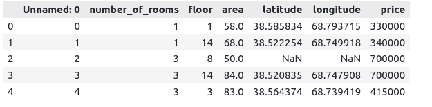
As you can see, our dataset contains an unnecessary column and some NULL values. Let us remove them from the dataset.

# removing the column
dushanbe.drop('Unnamed: 0', axis=1, inplace=True)
# removing null values
dushanbe.dropna(inplace=True)

Now let’s visualize the data set based on location and the price of the house. We can use a 3D plot from the Matplotlib library.

# importing the required module
import matplotlib.pyplot as plt
from mpl_toolkits.mplot3d import Axes3D
# size of the figure
fig = plt.figure(figsize=(15,8))
# 3-d plot
ax = fig.add_subplot(projection='3d')
# plotting
ax.scatter(dushanbe['latitude'], dushanbe['longitude'], dushanbe['price'])
ax.set_title('Location vs house prices')
plt.show()

Output:

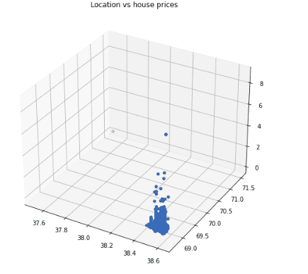
The output shows that most houses are located in one place, and the price changes as the location changes.

Splitting the dataset

Before training the model, we need to separate dataset features from outputs:

#get a copy of dataset exclude last column
Input = dushanbe.iloc[:, :-1].values 
#get array of dataset in column 2st
output = dushanbe.iloc[:, 5].values 

Now we can split the dataset into testing and training parts to evaluate the model afterward:

# Splitting the dataset into the Training data set and Testing data set
from sklearn.model_selection import train_test_split
# 30% data for testing, random state 1
X_train, X_test, y_train, y_test = train_test_split(Input, output, train_size=.7, random_state=1)

We have assigned 70% of the dataset for the training and the remaining 30% for the testing.

Training and testing the model

Let’s import the algorithm and start training on the training dataset.

# importing the module
from sklearn.linear_model import RANSACRegressor
# Initializing the model
Ransac = RANSACRegressor()
# training the model
Ransac.fit(X_train, y_train)

We’ve used the default parameters values. By default, the threshold value is the median absolute deviation of the target values, and the max number of iterations is 100.

Once the training is complete, we can see how many data points have been considered outliers by the model:

# inlier mask
inlier_mask = Ransac.inlier_mask_
print(inlier_mask)

Output:

So, the data points that are considered outliers are returned as False by the model. Let’s print the total number of outliers:

# inliers
inlier_mask = Ransac.inlier_mask_
# for loop to count
count = 0
for i in inlier_mask:
    if i==False:
        count +=1
# printing
print("Total datapoints were : ", len(inlier_mask))
print("Total outliers detected  were : ", count)

Output:

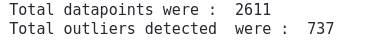
Each time you run the code, you will get different outliers because the algorithm selects the random points each time to find the best-fitted line, as we have learned in the section above.

Let’s predict the output by using the testing dataset:

# predicting
preditions_Ransac = Ransac.predict(X_test)

We can use the R²-score to evaluate the model’s performance, which shows how well the model is following the trend.

# Importing the required module
from sklearn.metrics import r2_score
# Evaluating the model
print('R score is :', r2_score(y_test, preditions_Ransac))

Output:

If the R-score is negative, the model has failed to follow the trends in the dataset. However, if the R-score is closer to 1, it means the model is trained so well.

Linear regression vs RANSAC

Let’s compare the model trained by the linear regression, which is highly affected by the outliers, and the model trained by the RANSAC, which is relying on inliers only. We will use a sample dataset about students where the input variable is the number of hours students spends studying, and the output class is the score they get out of 100. You can download the dataset from this link.

Importing and exploring the dataset

We will use the Pandas DataFrame to store the dataset and import it using the read_csv() method.

# importin pandas module
import pandas as pd
# importing the dataset
dataset = pd.read_csv("RANSAC_dataset.csv")

We can use the head() method to print out a few rows to get familiar with the dataset type.

# printing the head
dataset.head()

Output:

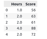
We can also check if our dataset contains null values or not:

# checking for null values
dataset.isnull().sum()

Output:

Note that our dataset doesn’t have any null values. Let’s now visualize the dataset to see how the data is organized:

# importing the module
import matplotlib.pyplot as plt
# setting the size
plt.figure(figsize=(15, 7))

# plotting scattered plot
plt.scatter(dataset['Hours'], dataset['Score'])
plt.show()

Output:

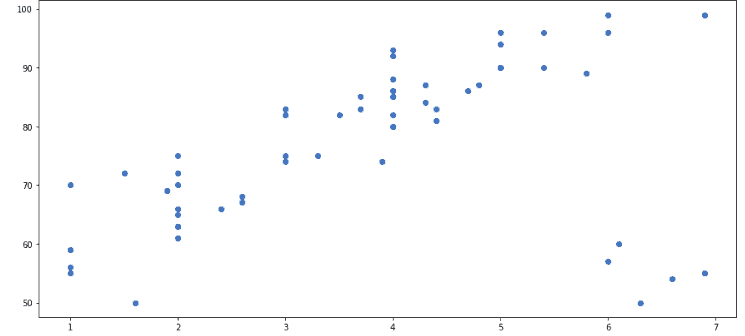
Pay attention, that the dataset contains some outliers which do not follow the visible trend. We will see how these outliers affect the training of the Linear Regression algorithm and how the RANSAC algorithm identifies them before training the model.

Training and visualizing the Linear Regression model

Let’s use the above dataset to train the Linear Regression model, but we need to split the dataset into input and output variables first:

#get a copy of dataset exclude last column
Input = dataset.iloc[:, :-1].values 
#get array of dataset in column 2st
output = dataset.iloc[:, 1].values 

Now we can train the model on the above dataset.

# Importing linear regression form sklear
from sklearn.linear_model import LinearRegression
# initializing the algorithm
regressor = LinearRegression()
# Fitting Simple Linear Regression to the Training set
regressor.fit(Input, output)

Once the training is complete, we can use the matplotlib module to visualize the best-fitted line by the Linear Regression model:

# importing the module
import matplotlib.pyplot as plt
# setting the size
plt.figure(figsize=(15, 7))
# ploting the training dataset in scattered graph
plt.scatter(Input, output, color='red')
# ploting the testing dataset in line line
plt.plot(Input, regressor.predict(Input), color='green')
# labeling the input and outputs
plt.title('Hours vs Score')
plt.xlabel('Hours')
plt.ylabel('Score')
# showing the graph
plt.show()

Output:

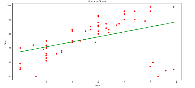
As you can see, the best-fitted line is a bit bent lower because of the outliers found on the plot’s left bottom.

Training and visualizing the RANSAC model

Now let’s train the RANSAC model on the same dataset.

# importing the module
from sklearn.linear_model import RANSACRegressor
# Initializing the model
ransac = RANSACRegressor()
# training the model
ransac.fit(Input, output)

Let’s visualize the best-fitted line of the RANSAC model.

# setting the size
plt.figure(figsize=(15, 7))
# ploting the training dataset in scattered graph
plt.scatter(Input, output, color='red')
# ploting the testing dataset in line line
plt.plot(Input, ransac.predict(Input), color='green')
# labeling the input and outputs
plt.title('Hours vs Score')
plt.xlabel('Hours')
plt.ylabel('Score')
# showing the graph
plt.show()

Output:

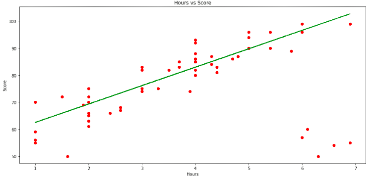
Notice that the best-fitted line of the RANSAC model is only based on the inliers, and it ignores the outliers while training,

Comparing Linear regression and the RANSAC model

We can now compare both models by providing testing input data. But first, let us visualize both models in one graph to see the difference:

# setting the size
plt.figure(figsize=(15, 7))
# ploting the training dataset in scattered graph
plt.scatter(Input, output, color='red')
# ploting the testing dataset in line line
plt.plot(Input, ransac.predict(Input), color='green', label="RANSAC")
plt.plot(Input, regressor.predict(Input), color='blue', label='Linear regression')
# labeling the input and outputs
plt.title('Hours vs Score')
plt.xlabel('Hours')
plt.ylabel('Score')
# showing the graph
plt.legend()
plt.show()

Output:

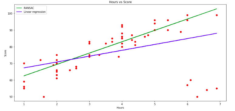
The plot clearly shows how the linear model has been affected by the presence of outliers. At the same time, the RANSAC model has been trained only on inliers. Also, the RANSAC model seems to follow the data trend, and it increases as the majority of data points increase (except outliers).

Let’s now take input data points to see the difference in the predictions. Let’s assume that a student is studying 6 hours a day as we want to predict their score using both models.

# defining the input data
input_data = [6]
# prediction of linear regression
predict_regression = regressor.predict([input_data])
# prediction of Ransac model
predict_ransac = ransac.predict([input_data])
# printing
print("The linear regression predictions is :", predict_regression)
print("\nThe RANSAC model's predicitions is  : ", predict_ransac)

Output:

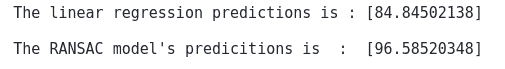
There is a clear difference between the predictions of both models. The Linear Regression predicted a lower score for a student because it was affected by the outliers. On the other hand, we trained the RANSAC model on only inliers, which is why it predicted a high score for the student.

Summary

Random Sample Consensus, or RANSAC, is an iterative method for estimating a mathematical model from a data set that contains outliers. The RANSAC algorithm identifies the outliers in a data set and estimates the desired model using data that does not contain outliers. In this article, we’ve covered the RANSAC regression algorithm and compared it with Linear Regression.