Simple Sklearn Ridge Regression Example In Python
In Machine Learning, regularization is a technique used to reduce errors by fitting the function appropriately on the given training set and avoiding overfitting. The Ridge and Lasso regressions are the most popular regularization techniques to generalize the model. This article demonstrates simple Sklearn Ridge Regression and Sklearn Lasso Regression implementation and how to apply them to solve regression problems using Python.
Table of contents
Getting started with Ridge Regression and Lasso Regression
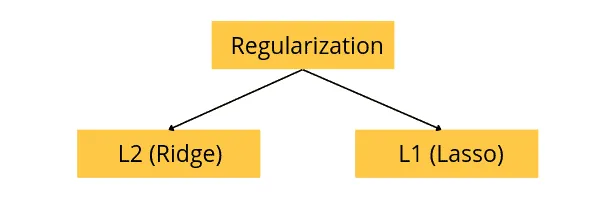
Ridge and Lasso Regressions are the two most common types of regularization techniques in regression methods. They are also known as L1 (the Lasso regression) and L2 (Ridge regression) regularizations.
Before going into the depth of Ridge and Lasso regression, let us first understand some terminologies we frequently use throughout the article.
What are overfitting and underfitting in Machine Learning?
We provide a bunch of data to train the Machine Learning models. We say a model is best fitted when it finds all the necessary patterns in the dataset. The process of plotting a series of data points and drawing the best-fit line to understand the relationship between the variables is called Data Fitting.
If we allow the model to train on the dataset many times, the model will find a lot of patterns, including unnecessary and noisy ones. The model will then learn well on the training dataset and fit very well, but then it will not be able to predict other datasets. So, in simple words, a scenario where the model learns from the data’s details and noise and tries to fit each data point on the curve is called overfitting.
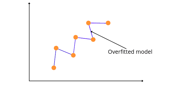
The figure above shows that the model is fitted for every point in our dataset. If a new data point is given, then the model curves may not correspond to the pattern in the new data, and the model may not be able to predict well.
While in some cases, you may not train the model a sufficient number of times on the dataset, and it fails to find the patterns. In such a case, again, the model will not fit appropriately into the training dataset and will fail to perform well on the new dataset. Underfitting is a scenario where a model can neither learn the relationship between variables nor predict the new data point.
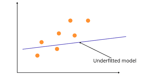
The figure above shows the under-fitted regression model. Such a model fails to perform on both known and unknown datasets. We can see that it has not fit properly into the given dataset and fails to find the patterns.
What is the difference between Bias and Variance?
A Bias occurs in a model when the model has limited flexibility to learn from the dataset. Such models pay very little attention to the training dataset and can’t find the trends. This type of modeling always leads to a high error in training and testing datasets. In other words, we can say that high bias causes underfitting in the model.
While variance defines the model’s sensitivity to a specific dataset, a model with a high variance pays a lot of attention to the training dataset and does not generalize; therefore, the prediction error is high. Such models usually perform well on training datasets but give high error rates on the testing datasets. In other words, high variance leads to the overfitting of the model.
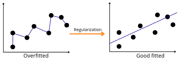
An optimal model is one in which the model is sensitive to the pattern in our model but at the same time can generalize to new data. This happens when Bias and Variance are both optimal. We can achieve such an optimal model in over or under-fitted models by using Regularization (Lasso and Ridge regression).
What is Regularization in Machine learning?
Regularization refers to techniques used to calibrate machine learning models to minimize the adjusted loss function and prevent overfitting or underfitting. Using regularization, we can fit our machine learning model appropriately on a given test set and reduce its errors.
Let us now learn how the L1 (the Lasso regression) and L2 (the Ridge regression) help to regularize the model.
How does Ridge regression work?
To understand how Ridge regression works, ensure you have a solid knowledge of Linear regression because they are similar. To get more information about Linear regression models, check out another article about using Linear Regression in Python.
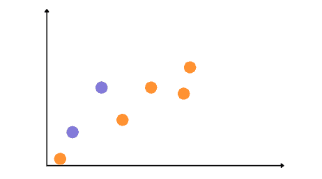
Let’s assume that we have the following dataset containing the training set (blue) and test set (orange):
We will get the following regression line if we apply Linear regression to the training dataset.
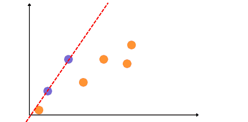
As you can see that the model has performed very well on the training dataset but fails to generalize the results for the testing dataset. In other words, the model is overfitted (low bias).
The main goal of Ridge regression is to find a new line that doesn’t fit well on the training data but reduces the error on the testing data. In other words, we will introduce a small amount of bias for the new fitted line on the training dataset to get a low variance for the testing data. For example, see the new fitted line (ridge regression) below, which reduces the variance compared to the previous overfitted line.
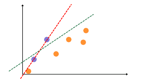
Notice that the new line does not perform well on the training dataset compared to the previous one. Still, it generalizes the results better on the testing data than the overfitted line. By starting with a slightly worse fitted line, Ridge regression can provide better long-term predictions.
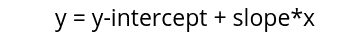
As we know, the simple linear equation uses the following mathematical equation to find the best-fitted line:
While the Ridge regression uses a slightly modified equation with the penalty term to find the new best-fitted line to introduce a small bias and reduce variance, the penalty term, also known as the penalty function or cost function, contains lambda and slope square, as shown below.

Here the slope-square adds a cost function to the linear equation while the lambda determines how severe that penalty is. o see how the value of lambda affects the fitted line, see the diagrams below:
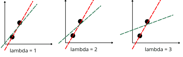
Notice that the slope decreases as we increase the lambda value, which means the best-fitted line becomes less sensitive to the input values. Lambda can be any value from 0 to infinity. The larger the value, the smaller the slope of the fitted line will be.
How does Lasso regression work?
The word “LASSO” denotes the Least Absolute Shrinkage and Selection Operator. The Lasso regression model uses the shrinkage technique. It is also known to be one of the spare models (i.e., models with fewer parameters),
The Lasso regression works very similarly to the Ridge regression with a slight change in the training equation. The Lasso regression uses the following mathematical equation to find the best-fitted line.

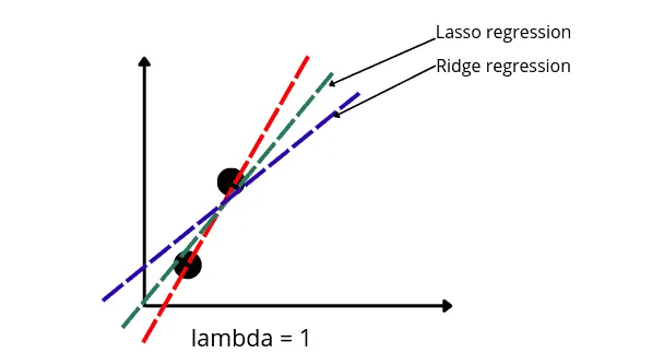
Note that instead of squaring the slope for the penalty term, the Lasso regression takes the absolute value of the slope (The absolute value will return all positive values). That means for the same value of lambda, the Lasso regression will produce less bias than the Ridge regression, as shown below:
Using Ridge and Lasso regressions in Python
We will use Ridge and Lasso regression models to find the fitted line. In this section, we will be using a dataset about house pricing. The input variables (or independent variables) contain the number of floors, rooms, area, and location of the house, and the output variable or the target variable is the price of the house. You can get access to the dataset from this link.
Before going to the implementation part, ensure that you have installed the following Python modules, as we will use them in the upcoming sections.
- sklearn
- pandas
- numpy
- matplotlib
- plotly
You can install the required modules by running the following commands in the cell of the Jupyter notebook.
%pip install sklearn
pip install pandas
pip install numpy
pip install matplotlib
pip install plotly
Once the modules are installed successfully, we can move to the implementation part.
Importing and exploring the dataset
We will use the read_csv() method of the Pandas library to import the dataset:
# Import standard modules
import io
import urllib3
# importing the Pandas module
import pandas as pd
# Download dataset from our site
http = urllib3.PoolManager()
r = http.request('GET', 'https://hands-on.cloud/wp-content/uploads/2022/04/Dushanbe_house.csv')
# importing the dataset
Dushanbe = pd.read_csv(io.StringIO(r.data.decode('utf-8')))
# get dataset demo
Dushanbe.head()
Output:
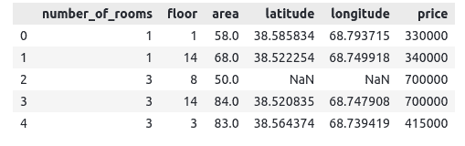
Notice that we have five input variables and one target variable. As you can see, there are some null values, so let us now remove those null values.
# removing null values
Dushanbe.dropna(axis=0, inplace=True)
# display null values if exist
Dushanbe.isnull().sum()
Output:
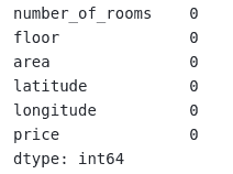
As you can see, now there are no null values.
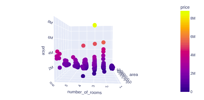
Let us now visualize different input data with the price of the houses. We will first visualize the number of rooms and area vs. the price of the home.
# importing the plotly module
import plotly.express as px
# plotting 3-d plot
fig = px.scatter_3d(Dushanbe, x='number_of_rooms', y='area', z='price',
              color='price')
fig.show()
Output:
Implementing Sklearn Ridge Regression
In Ridge Regression, the loss function is the linear least squares function, and the L2-norm gives the regularization.
Now we will apply the Ridge regression to the dataset. But first, let us split the dataset into an independent variable and a dependent variable.
# taking the columns from the dataset
columns = Dushanbe.columns
# storing the input and output variables
Inputs = Dushanbe[columns[0:-1]]
#dependent variable
outputs = Dushanbe[columns[-1]]
Once we divide the dataset into input and output ports, we can then split the dataset into training and test parts.
# importing the module
from sklearn.model_selection import train_test_split
# splitting into test data and traind data for ridge regression
X_train, X_test, y_train, y_test = train_test_split(Inputs, outputs, test_size=0.25, random_state=42)
Now we will import the Ridge algorithm from the sklearn module. We will fix the lambda value to 0.9.
from sklearn.linear_model import Ridge
# alpha parameter 0.9 and initializing ridge regression
model = Ridge(alpha=0.9)
# ridge function
model.fit(X_train, y_train)
Once the training is complete, we can use the testing data to make predictions.
# predictive models of ridge regression models
y_pred = model.predict(X_test)
Once the predictions are completed, we can find the r-2 score to see how well the model makes predictions.
# Importing the required module
from sklearn.metrics import r2_score
# Evaluating model performance
print('R-square score is :', r2_score(y_test, y_pred))
Output:

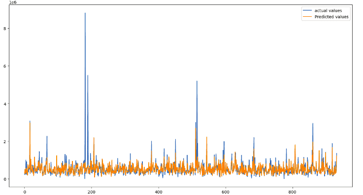
Let us now visualize the predictions and the actual values to get more information related to predictions.
# importing the module
import matplotlib.pyplot as plt
# fitting the size of the plot
plt.figure(figsize=(15, 8))
# plotting the graphs for actual-value and predicted values
plt.plot([i for i in range(len(y_test))],y_test, label="actual-values")
plt.plot([i for i in range(len(y_test))],y_pred, label="Predicted values")
# showing the plotting of predictive modelling technique
plt.legend()
plt.show()
Output:

As we can see, our model has performed well and followed the trend to give an accurate prediction.
You can also use other regression evaluation matrices to evaluate the performance of Lasso and Ridge regression, like mean squared error, absolute error, etc.
Implementing Sklearn Lasso Regression
Now we will apply the Lasso regression to the same split dataset. Let’s first import the algorithm from the sklearn module.
# lasso regression implementation
from sklearn.linear_model import Lasso
# lasso regression select initialization
lasso_model = Lasso(alpha=0.9)
# training the lasso regression model
lasso_model.fit(X_train, y_train)
Once the training is complete, we can make predictions using the testing dataset.
# predictive model of lasso regression with test data
lasso_predictions = lasso_model.predict(X_test)
Let us now calculate the r-square of the lasso model.
# Evaluating model performance to see accurate model
print('R-square score is :', r2_score(y_test, lasso_predictions))
Output:

Let us also visualize the Lasso regression model’s predictions and real values.
# fitting the size of the plot
plt.figure(figsize=(15, 8))
# plotting the graphs for observed value and real values
plt.plot([i for i in range(len(y_test))],y_test, label="actual-values")
plt.plot([i for i in range(len(y_test))],lasso_predictions, label="Predicted values")
# showing the plotting of lasso regression
plt.legend()
plt.show()
Output:
As you can see, the model has performed well in making an accurate prediction.
Summary
Lasso and ridge regression are powerful techniques generally used to create economic models in the presence of many features. They help us create an optimal model (either overfitted or under fitted). In this article, we learn how the Ridge and Lasso regression works. We also implemented the Lasso and Ridge regression using Python programming language.
