SVM Python – Easy Implementation of SVM algorithm
Machine Learning opens endless opportunities to develop computer systems that can learn and adapt without explicit instructions, analyze and visualize inference data patterns using algorithms and statistical models. SVM Python algorithm implementation helps solve classification and regression problems, but its real strength is in solving classification problems.
This article covers the Support Vector Machine algorithm implementation, explains the mathematical calculations behind it, and give you examples of its implementation and performance evaluation using the sklearn Python module.
Table of contents
The Support-vector machine (SVM) algorithm is one of the Supervised Machine Learning algorithms. Supervised learning is a type of Machine Learning where the model is trained on historical data and makes predictions based on the trained data. The historical data contains the independent variables (inputs) and dependent variables (outputs). The algorithm finds the relation between these variables to make predictions using labeled data.
Overview of the SVM algorithm
Support Vector Machine (SVM), also known as Support Vector Classification, is a supervised and linear Machine Learning technique typically used to solve classification problems. SVR stands for Support Vector Regression and is a subset of SVM that uses the same ideas to tackle regression problems. SVM also supports the kernel method called the kernel SVM, which allows us to tackle non-linearity.
The primary use case for SVM is classification, but it can solve classification and regression problems. SVM constructs a hyperplane (see the picture below) in multidimensional space to separate different classes. It iteratively generates the best hyperplane to minimize classification error. The goal of SVM is to find a maximum marginal hyperplane (MMH) that splits a dataset into classes as evenly as possible.
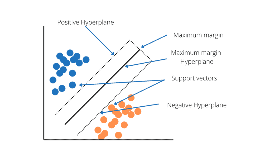
Support Vectors are data points closest to the hyperplane called support vectors. These points will define the separating line better by calculating margins and are more relevant to the construction of the classifier.
A hyperplane is a decision plane that separates objects with different class memberships.
Margin is the distance between the two lines on the class points closest to each other. It is calculated as the perpendicular distance from the line to support vectors or nearest points. The bold margin between the classes is good, whereas a thin margin is not good.
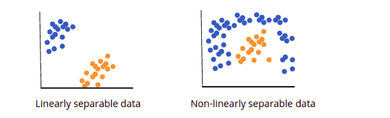
Depending on the type of data, there are two types of Support Vector Machines:
- Linear SVM or Simple SVM is used for data that is linearly separable. A dataset is termed linearly separable data if it can be classified into two classes using a single straight line, and the classifier is known as the linear SVM classifier. It’s most commonly used for tasks involving linear regression and classification.
- Nonlinear SVM or Kernel SVM also known as Kernel SVM, is a type of SVM that is used to classify nonlinearly separated data, or data that cannot be classified using a straight line. It has more flexibility for nonlinear data because more features can be added to fit a hyperplane instead of a two-dimensional space.
Explanation of the SVM algorithm
Let’s look at the example and see how the SVM algorithm will classify fruits into apple or orange categories. The classification will be based on the characteristics of the fruits we provide to the machine. For example, it can be the fruit’s size, shape, or weight. The more features we consider, the easier it is to identify and distinguish both.
How would a machine using the SVM algorithm classify a new fruit as either apple or orange based on the training data(apples and oranges) observed and labeled?
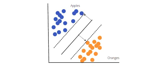
The objective of SVM is to draw a line that best separates the two classes of data points. SVM produces a line that cleanly divides the two classes (in our case, apples and oranges). There are many other ways to construct a line that separates the two classes, but in SVM, the margins and support vectors are used.
The image above shows that the margin separates the two dotted lines. The larger this margin is, the better the classifier will be. The data points that each dotted line passes through are the support vectors. These points are support vectors since they help define the margins and the classifier. These support vectors are the data points closest to the border of either of the classes and have a chance of belonging to one of them.
The SVM then creates a hyperplane with the highest margin, which in this example is the bold black line that separates the two classes and is at the optimum distance between them.
SVM Kernels
Some problems can’t be solved using a linear hyperplane because they are non-linearly separable. In such a situation, SVM uses a kernel trick to transform the input space into a higher-dimensional space.
There are different types of SVM kernels depending on the kind of problem.
Linear Kernel is a regular dot product for two observations. The sum of the multiplication of each pair of input values is the product of two vectors.

Polynomial Kernel is a more generalized form of Linear Kernel. The polynomial Kernel can tell if the input space is curved or nonlinear.

The d is the degree of the polynomial. If the d = 1, then it is similar to the linear transformation. The degree needs to be manually specified in the learning algorithm.
Radial Basis Function Kernel can map an input space into an infinite-dimensional space.

Here gamma is a parameter, which ranges from 0 to 1. A higher gamma value will perfectly fit the training dataset, which causes over-fitting. The gamma = 0.1 is considered to be a good default value. The gamma value again needs to be manually specified in the learning algorithm.
SVM Python algorithm – Binary classification
Let’s implement the SVM algorithm using Python programming language. We will use AWS SageMaker services and Jupyter Notebook for implementation purposes. Before jumping into the implementation, ensure that you have installed all the required modules:
- sklearn
- pandas
- seaborn
- matplotlib
- numpy
You can install these modules right from your Jupyter Notebook by running pip command in its cells:
% pip install sklearn
% pip install pandas
% pip install seaborn
% pip install matplotlib
% pip install numpy
Once you’ve installed modules successfully, we can jump to the implementation part.
Binary Data set for SVM algorithm
Let’s use a binary dataset to train our model. In this case, we will use customer data about whether the customer had purchased a product.
You can download the dataset from here.
Import the required modules:
# importing the libraries
import matplotlib.pyplot as plt
import pandas as pd
import seaborn as sns
The next step is to import the data set and divide it into input and output variables.
# importing the dataset
dataset = pd.read_csv('customer_purchases.csv')
# split the data into inputs and outputs
X = dataset.iloc[:, [0,1]].values
y = dataset.iloc[:, 2].values
We can print out the target/output class to verify that our data is a binary set (containing only two output categories).
# printing the target values
print(dataset.Purchased)
Output:
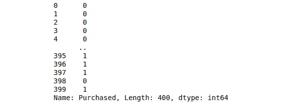
Notice that the output class contains either 1 or 0, showing whether the customer had purchased the product or not.
The next thing we can do as a part of data pre-processing is visually seen the number of those output classes.
# importing the required modules for data visualization
import matplotlib.pyplot as plt
import chart_studio.plotly as py
import plotly.graph_objects as go
import plotly.offline as pyoff
import pandas as pd
# importing the dats set
data = pd.read_csv('SVM_data.csv')
# counting the total output data from purchased column
target_balance = data['Purchased'].value_counts().reset_index()
# dividing the output classes into two sections
target_class = go.Bar(
    name = 'Target Balance',
    x = ['Not-Purchased', 'Purchased'],
    y = target_balance['Purchased']
)
# ploting the output classes
fig = go.Figure(target_class)
pyoff.iplot(fig)
output:
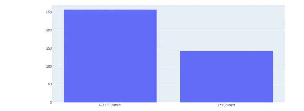
The shows that more people have not purchased the product.
Training and testing linear SVM model
Once we are done with the pre-processing of the data, we can move into the splitting part to divide the data into the testing and training parts.
# training and testing data
from sklearn.model_selection import train_test_split
# assign test data size 25%
X_train, X_test, y_train, y_test =train_test_split(X, y, test_size=0.25, random_state=0)
We have assigned 25% of the data to the testing and 75% to the training parts. That means our model will use 75% of the original data for training, and the remaining portion will be used to test the model to know how accurately our model predicts the output class.
Before feeding the training data to our model, we need to scale the given data so that the outlier will not affect the output class.
# importing StandardScaler
from sklearn.preprocessing import StandardScaler
# scalling the input data
sc_X = StandardScaler()
X_train = sc_X.fit_transform(X_train)
X_test = sc_X.fit_transform(X_test)
Notice that scaling is only applied to the input/independent variables. Once the scaling is done, our data is then ready to be used to train our model.
# importing SVM module
from sklearn.svm import SVC
# kernel to be set linear as it is binary class
classifier = SVC(kernel='linear')
# traininf the model
classifier.fit(X_train, y_train)
After the training, we must provide the testing data to see how well our model predicts.
# testing the model
y_pred = classifier.predict(X_test)
We’re storing predicted outputs in the y_pred variable. We can then use these predicted outputs to find the accuracy of our model.
# importing accuracy score
from sklearn.metrics import accuracy_score
# printing the accuracy of the model
print(accuracy_score(y_test, y_pred))
Output:

Visualizing trained data
Let’s visualize the model trained by the Linear Kernel to see how the model has been trained visually.
# importing the modules
import numpy as np
import matplotlib.pyplot as plt
from matplotlib.colors import ListedColormap
# plotting the fgiure
plt.figure(figsize = (7,7))
# assigning the input values
X_set, y_set = X_train, y_train
# ploting the linear graph
X1, X2 = np.meshgrid(np.arange(start = X_set[:, 0].min() - 1, stop = X_set[:, 0].max() + 1, step = 0.01), np.arange(start = X_set[:, 1].min() - 1, stop = X_set[:, 1].max() + 1, step = 0.01))
plt.contourf(X1, X2, classifier.predict(np.array([X1.ravel(), X2.ravel()]).T).reshape(X1.shape), alpha = 0.75, cmap = ListedColormap(('black', 'white')))
plt.xlim(X1.min(), X1.max())
plt.ylim(X2.min(), X2.max())
# ploting scattered graph for the values
for i, j in enumerate(np.unique(y_set)):
plt.scatter(X_set[y_set == j, 0], X_set[y_set == j, 1], c = ListedColormap(('red', 'blue'))(i), label = j)
# labeling the graph
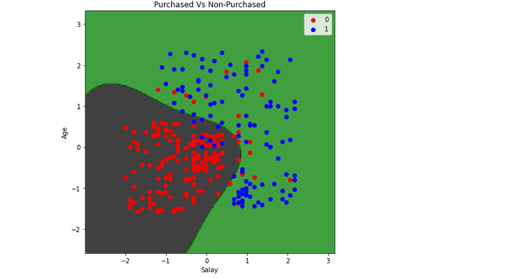
plt.title('Purchased Vs Non-Purchased')
plt.xlabel('Salay')
plt.ylabel('Age')
plt.legend()
plt.show()Output:

Notice that there is a linear boundary between the two classes because we have specified the Kernel to be linear.
Visualising predicted data
Similarly, we can also visualize the predictions of our model, bypassing the testing dataset.
# ploting graph of size 7,7
plt.figure(figsize = (7,7))
# assigning the testing dataset
X_set, y_set = X_test, y_test
# ploting the predicted graph
X1, X2 = np.meshgrid(np.arange(start = X_set[:, 0].min() - 1, stop = X_set[:, 0].max() + 1, step = 0.01),np.arange(start = X_set[:, 1].min() - 1, stop = X_set[:, 1].max() + 1, step = 0.01))
plt.contourf(X1, X2, classifier.predict(np.array([X1.ravel(), X2.ravel()]).T).reshape(X1.shape),alpha = 0.75, cmap = ListedColormap(('black', 'white')))
plt.xlim(X1.min(), X1.max())
plt.ylim(X2.min(), X2.max())
# plorting scattred graph for the testing values
for i, j in enumerate(np.unique(y_set)):
plt.scatter(X_set[y_set == j, 0], X_set[y_set == j, 1],c = ListedColormap(('red', 'blue'))(i), label = j)
# labelling the graphe
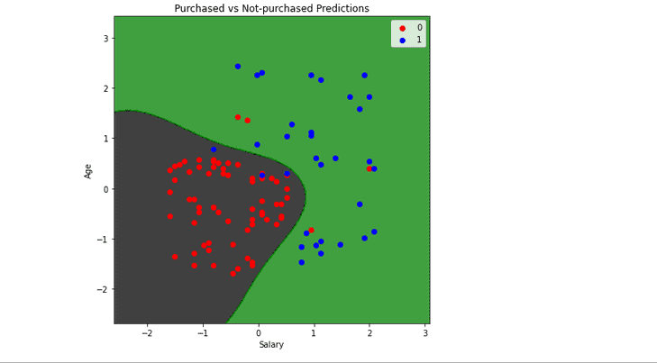
plt.title('Purchased vs Not-purchased Predictions')
plt.xlabel('Salary')
plt.ylabel('Age')
plt.legend()
plt.show()Output:

You can consider any testing point in the black area as Not-purchased and any point in the while area as Purchased.
Training and testing nonlinear SVM model
We know that the Linear Kernel performs best when the data is linear, but we use other kernels when the information is nonlinear. Let’s train our model using the Radial Basis Function kernel and visualize the results.
First, we will train the model and test it to see its accuracy.
# importing SVM module
from sklearn.svm import SVC
# kernel to be set radial bf
classifier1 = SVC(kernel='rbf')
# traininf the model
classifier1.fit(X_train, y_train)
# testing the model
y_pred = classifier1.predict(X_test)
# importing accuracy score
from sklearn.metrics import accuracy_score
# printing the accuracy of the model
print(accuracy_score(y_test, y_pred))
Output:

Note: the accuracy of our model has increased because the Radial Basis Function kernel has performed well as the data we not linear.
Visualizing trained data(Radial Basis Function kernel)
Let’s visualize the classifier trained by the Radial Basis Function kernel.
# plotting the fgiure
plt.figure(figsize = (7,7))
# assigning the input values
X_set, y_set = X_train, y_train
# ploting the linear graph
X1, X2 = np.meshgrid(np.arange(start = X_set[:, 0].min() - 1, stop = X_set[:, 0].max() + 1, step = 0.01), np.arange(start = X_set[:, 1].min() - 1, stop = X_set[:, 1].max() + 1, step = 0.01))
plt.contourf(X1, X2, classifier1.predict(np.array([X1.ravel(), X2.ravel()]).T).reshape(X1.shape), alpha = 0.75, cmap = ListedColormap(('black', 'green')))
plt.xlim(X1.min(), X1.max())
plt.ylim(X2.min(), X2.max())
# ploting scattered graph for the values
for i, j in enumerate(np.unique(y_set)):
    plt.scatter(X_set[y_set == j, 0], X_set[y_set == j, 1], c = ListedColormap(('red', 'blue'))(i), label = j)
# labeling the graph
plt.title('Purchased Vs Non-Purchased')
plt.xlabel('Salay')
plt.ylabel('Age')
plt.legend()
plt.show()
Output:
Visualizing predictions (Radial Basis Function kernel)
Let us now visualize the predictions made by the Radial Basis Function kernel. The process will be the same with the same code, except for the dataset.
# ploting graph of size 7,7
plt.figure(figsize = (7,7))
# assigning the testing dataset
X_set, y_set = X_test, y_test
# ploting the predicted graph
X1, X2 = np.meshgrid(np.arange(start = X_set[:, 0].min() - 1, stop = X_set[:, 0].max() + 1, step = 0.01),np.arange(start = X_set[:, 1].min() - 1, stop = X_set[:, 1].max() + 1, step = 0.01))
plt.contourf(X1, X2, classifier1.predict(np.array([X1.ravel(), X2.ravel()]).T).reshape(X1.shape),alpha = 0.75, cmap = ListedColormap(('black', 'green')))
plt.xlim(X1.min(), X1.max())
plt.ylim(X2.min(), X2.max())
# plorting scattred graph for the testing values
for i, j in enumerate(np.unique(y_set)):
    plt.scatter(X_set[y_set == j, 0], X_set[y_set == j, 1],c = ListedColormap(('red', 'blue'))(i), label = j)
# labelling the graphe
plt.title('Purchased vs Not-purchased Predictions')
plt.xlabel('Salary')
plt.ylabel('Age')
plt.legend()
plt.show()
Output:
Any data point in the black area will be classified as not-purchased, and in the green space will be classified as purchased. Using the same method and code, you can also use the polynomial Kernel and visualize its classifier and predictions.
Evaluation of SVM algorithm performance for binary classification
A confusion matrix is a summary of prediction results on a classification problem. The correct and incorrect predictions are summarized with count values and broken down by each class. The confusion matrix helps us calculate our model’s accuracy, recall, precision, and f1-score. You can learn more about the confusion matrix from the “Implementing KNN classification using Python” article.
Linear Kernel
Let us first visualize the confusion matrix of our model trained by using a Linear Kernel.
# importing the required modules
import seaborn as sns
from sklearn.metrics import confusion_matrix
# passing actual and predicted values
cm = confusion_matrix(y_test, y_pred, labels=classifier.classes_)
# true Write data values in each cell of the matrix
sns.heatmap(cm, annot=True)
plt.savefig('confusion.png')
Output:
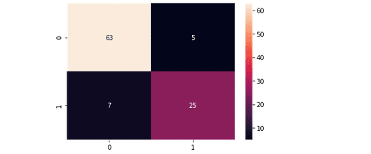
This output shows that 63 of the Non-purchased class were classified correctly, and 25 of the purchased were classified correctly.
# importing classification report
from sklearn.metrics import classification_report
# printing the report
print(classification_report(y_test, y_pred))
The accuracy report for the moel trained by using Linear Kernel is as follows:
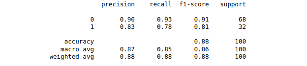
Nonlinear kernel
Let us now find the confusion matrix for our model trained using the Radial Basis Function kernel.
# importing the required modules
import seaborn as sns
from sklearn.metrics import confusion_matrix
# passing actual and predicted values
cm = confusion_matrix(y_test, y_pred, labels=classifier1.classes_)
# true Write data values in each cell of the matrix
sns.heatmap(cm,annot=True)
plt.savefig('confusion.png')
Output:
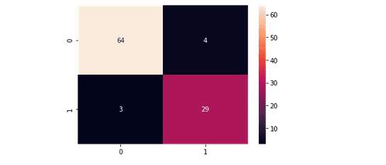
This time we get 64 of the non-purchased classified correctly and 29 purchased class classified correctly. We can also print out the classification report for both of our models.
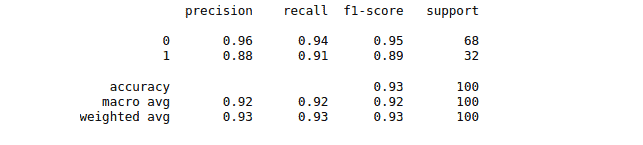
And the classification report for the model trained by using the Radial Basis Function kernel is:
SVM Python algorithm – multiclass classification
Multiclass classification is a classification with more than two target/output classes. For example, classifying a fruit as either apple, orange, or mango belongs to the multiclass classification category. We will use a Python build-in data set from the module of sklearn. We will use a dataset named “wines” formed based on the results of a chemical analysis of wines grown in the same region in Italy but derived from three different cultivars.
The dataset consists of 13 features (alcohol, malic_acid, ash, alcalinity_of_ash, magnesium, total_phenols, flavanoids, nonflavanoid_phenols, proanthocyanins, color_intensity, hue, od280/od315_of_diluted_wines, proline) and type of wine cultivar. This data has three types of wines: Class_0, Class_1, and Class_3. Let us now start pre-processing the data before feeding it to our model.
Training dataset for multiclass classification using SVM algorithm
Let us first import the data set from the sklearn module:
# import scikit-learn dataset library
from sklearn import datasets
# load dataset
dataset = datasets.load_wine()
Let us get a little bit familiar with the dataset. First, we will print the target and feature attributes headings.
# print the names of the 13 features
print ("Inputs: ", dataset.feature_names)
# print the label type of wine(class_0, class_1, class_2)
print ("Outputs: ", dataset.target_names)
Output:

We can also verify that it is multiclass classification data by printing out the target values.
# print the wine labels
print (dataset.target)
Output:
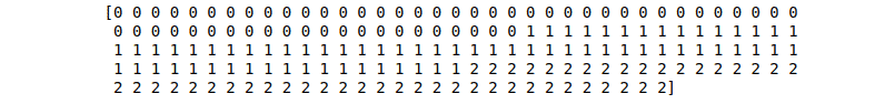
Note: there are three output classes.
Training and testing model using multiclass data
The next step is to split our dataset into training and testing parts so that we can evaluate the model’s performance later.
# import train_test_split function
from sklearn.model_selection import train_test_split
# input and outputs
inputs = dataset.data
outputs = dataset.target
# Split dataset into training set and test set
X_train, X_test, y_train, y_test = train_test_split(inputs, outputs, test_size=0.3, random_state=1)
We have assigned 70% of the data to the training part and the remaining 30% to the testing part.
Feed the training data to our model and train it using the SVM algorithm.
# importing SVM module
from sklearn.svm import SVC
# kernel to be set radial bf
classifier1 = SVC(kernel='rbf')
# traininf the model
classifier1.fit(X_train,y_train)
# testing the model
y_pred = classifier1.predict(X_test)
# importing accuracy score
from sklearn.metrics import accuracy_score
# printing the accuracy of the model
print(accuracy_score(y_test, y_pred))
Output:

We have used the Radial Basis Function kernel. Let us know to train our model using linear kerne to see the difference in prediction accuracy.
# importing SVM module
from sklearn.svm import SVC
# kernel to be set radial bf
classifier1 = SVC(kernel='linear')
# traininf the model
classifier1.fit(X_train,y_train)
# testing the model
y_pred = classifier1.predict(X_test)
# importing accuracy score
from sklearn.metrics import accuracy_score
# printing the accuracy of the model
print(accuracy_score(y_test, y_pred))
Output:

Note: there is a considerable improvement in the accuracy by changing the kernel type.
Visualizing the SVM for multiclass classification
Now let us visualize the working and classification process of the SVM algorithm on multi-labeled data. We will take only the two features and the target values. We will visualize the SVM algorithm using different kernels, which will help us understand the working of different Kernels in more detail.
Let us first visualize the SVM algorithm, which uses a Linear Kernel.
# import some data to play with
from sklearn import svm
# we only take the first two features.
X = dataset.data[:, :2]
y = dataset.target
# create a mesh to plot in
x_min, x_max = X[:, 0].min() - 1, X[:, 0].max() + 1
y_min, y_max = X[:, 1].min() - 1, X[:, 1].max() + 1
h = (x_max / x_min)/100
xx, yy = np.meshgrid(np.arange(x_min, x_max, h),
 np.arange(y_min, y_max, h))
# SVM regularization parameter
C = 1.0

#kernel is set to be linear
svc = svm.SVC(kernel='linear', C=1,gamma='auto').fit(X, y)
#Ploting part
plt.subplot(1, 1, 1)
Z = svc.predict(np.c_[xx.ravel(), yy.ravel()])
Z = Z.reshape(xx.shape)
plt.contourf(xx, yy, Z, cmap= ListedColormap(('blue', 'green', 'gray')), alpha=0.8)
plt.scatter(X[:, 0], X[:, 1], c = y, cmap=plt.cm.Paired)
plt.xlabel('First_feature')
plt.ylabel('Second_Feature')
plt.xlim(xx.min(), xx.max())
plt.title('SVC with linear kernel')
plt.show()
Output:
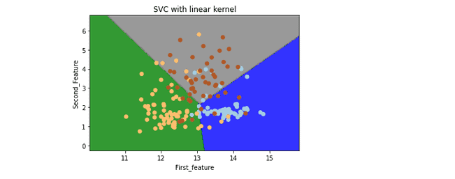
Now let us visualize the SVM classifier when the Kernel is polynomial for multiclass labeled data.
Note: the boundaries between different labels are linear, so we need to change the Kernel to the poly in our code to fix that.
# Kernel is set to be poly
svc = svm.SVC(kernel='poly', C=1,gamma='auto').fit(X, y)
#ploting part
plt.subplot(1, 1, 1)
Z = svc.predict(np.c_[xx.ravel(), yy.ravel()])
Z = Z.reshape(xx.shape)
plt.contourf(xx, yy, Z, cmap= ListedColormap(('blue', 'green', 'gray')), alpha=0.8)
plt.scatter(X[:, 0], X[:, 1], c = y, cmap=plt.cm.Paired)
plt.xlabel('First_feature')
plt.ylabel('Second_Feature')
plt.xlim(xx.min(), xx.max())
plt.title('SVC with kernel poly')
plt.show()
Output:
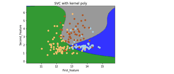
Note: this time, boundaries are not straight lines. They are curved because we have used a polynomial kernel.
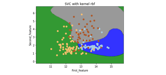
Let’s visualize the classifier by setting the Kernel as a Radial Basis Function.
# Kernel is set to be rbf
svc = svm.SVC(kernel='rbf', C=1,gamma='auto').fit(X, y)
#ploting part
plt.subplot(1, 1, 1)
Z = svc.predict(np.c_[xx.ravel(), yy.ravel()])
Z = Z.reshape(xx.shape)
plt.contourf(xx, yy, Z, cmap= ListedColormap(('blue', 'green', 'gray')), alpha=0.8)
plt.scatter(X[:, 0], X[:, 1], c = y, cmap=plt.cm.Paired)
plt.xlabel('First_feature')
plt.ylabel('Second_Feature')
plt.xlim(xx.min(), xx.max())
plt.title('SVC with kernel rbf')
plt.show()
Output:
Evaluation of SVM for multiclassification
Now let us evaluate the models by using a confusion matrix. The number of rows/columns will equal the number of target values.
# Importing the required modules
import seaborn as sns
from sklearn.metrics import confusion_matrix
# passing actual and predicted values
cm = confusion_matrix(y_test, y_pred)
# true Write data values in each cell of the matrix
sns.heatmap(cm,annot=True)
plt.savefig('confusion.png')
The confusion matrix for the model trained by using the Radial Basis Function kernel is as follows:
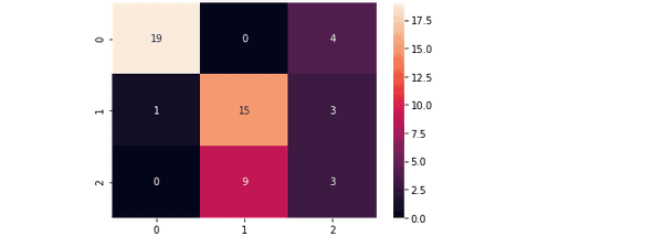
And the confusion matrix for the model trained by using Linear Kernel is:
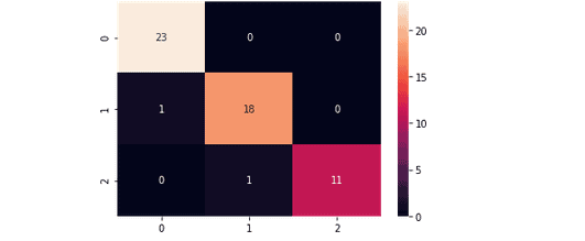
Notice that the Linear Kernel predicted very well, which means our data is more linearly related.
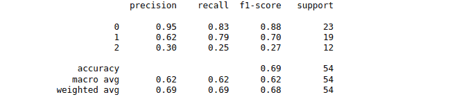
Now let us print out the classification score for both models, which will further help us evaluate the models.
# Importing classification report
from sklearn.metrics import classification_report
# printing the report
print(classification_report(y_test, y_pred))
The classification report for the model trained by using Radial Basis Function is as follows:
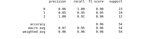
While the classification report for the model trained by the Linear Kernel is as follows
SVM algorithm using Python and AWS SageMaker Studio
Let’s implement the SVM algorithm in Python on AWS SageMaker Studio, where we are using the Python version 3.7.10.
First, we must import the dataset, split it and train our model. This time we will use the polynomial kernel method to train our model.
# importing the libraries
import matplotlib.pyplot as plt
import pandas as pd
# importing the dataset
dataset = pd.read_csv('SVM_data.csv')
# split the data into inputs and outputs
X = dataset.iloc[:, [0,1]].values
y = dataset.iloc[:, 2].values
# training and testing data
from sklearn.model_selection import train_test_split
# assign test data size 25%
X_train, X_test, y_train, y_test =train_test_split(X,y,test_size= 0.25, random_state=0)
# importing standardScaler
from sklearn.preprocessing import StandardScaler
# scalling the input data
sc_X = StandardScaler()
X_train = sc_X.fit_transform(X_train)
X_test = sc_X.fit_transform(X_test)
# importing SVM module
from sklearn.svm import SVC
# kernel to be set linear as it is binary class
# classifier = SVC(kernel='rbf')
classifier = SVC(kernel='poly')
# traininf the model
classifier.fit(X_train,y_train)
# testing the model
y_pred = classifier.predict(X_test)
# importing accuracy score
from sklearn.metrics import accuracy_score
# printing the accuracy of the model
print(accuracy_score(y_test, y_pred))
Output:

Summary
Support Vector Machine is a Supervised learning algorithm to solve classification and regression problems for linear and nonlinear problems. In this article, we’ve described the implementation of the SVM algorithm using Python and covered its evaluation using a confusion matrix and classification score. We’ve used the AWS SageMaker Studio and Jupyter Notebook for implementation and visualization.
