TensorFlow Regression Model – Simple example
Artificial Neural Networks (ANNs) are computational models inspired by the brain. These models perform tasks that are difficult for traditional computer programs, such as image recognition and natural language processing. ANNs are composed of many interconnected processing nodes or neurons that can learn to perform complex tasks by modifying the strength of the connections between them. TensorFlow is an open-source library for Machine Learning developed by Google Brain. It offers a variety of tools, libraries, and resources that allow developers to build and train Machine Learning models.
TensorFlow can be used for various tasks, such as classification, natural language processing, and time series analysis. In this article, we will use TensorFlow to build a Neural Network model to help us solve a regression problem and predict the continuous output values. We will also learn how to evaluate a TensorFlow Regression model and how to improve its predictions.
Table of contents
We assume you have a basic understanding of Artificial Neural Networks and the TensorFlow implementation. To get familiar with the basic concepts, you can check the articles Introduction to Neural Networks and Introduction to TensorFlow. You can also refer to the Python Linear Regression – Simple Tutorial to learn how to handle regression problems in Machine Learning.
Overview of Neural Network Regression
A Neural Network is a series of algorithms that detect basic patterns in a dataset. The Neural Network works similarly to the neural network in the human brain. A neuron in a neural network is a mathematical function that searches for and classifies patterns according to a specific architecture. A simple Neural Network consists of three layers:
- Input layer
- Hidden Layers
- Output Layer
In the case of regression, the output layer contains only one node, as shown below:
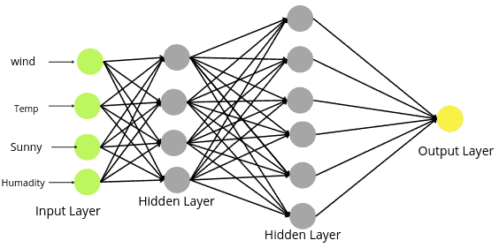
In the case of a regression problem, any activation function can be applied in the hidden layer ( except softmax), but the output layer should have a Linear activation function.
Creating a TensorFlow Regression model
Now, we will dive into the practical part of Neural Networks and create a regression model. In the first part of the implementation, we will learn how to create Neural Network regression by taking a sample dataset. Then in the second part, we will solve a real regression problem using the ANN regression model.
There are three main steps to creating a model in TensorFlow:
- Creating a model: The first step is initializing and creating a model. In our case, we will create a regression model.
- Compiling the model: Here, we define how to measure the model’s performance and specify the optimizer.
- Fitting the model: This is the training step of the model on the training dataset.
Before creating the model for the regression problem, let us first create a sample regression dataset.
Creating regression dataset
For demonstration purposes, we will use NumPy to create a sample dataset.
# Importing the numpy module
import numpy as np

# creating custom data/ x and y values
X = np.arange(-210, 210, 3)
y = np.arange(-200, 220, 3)
Let us now print out the shape of the X and y. For any model, the shape of the X and y should be the same.
# shape of created data
X.shape, y.shape
Output:
As you can see, both datasets have the same shape.
Let us now visualize the dataset to see how they are distributed in a two-dimensional graph.
# importing the matplotlib module
import matplotlib.pyplot as plt
# fixing the size of the plot
plt.figure( figsize = (12,6))
# plotting scattered plot of linear data
plt.scatter(X, y, label = 'Dataset')
plt.legend()
plt.show()
Output:
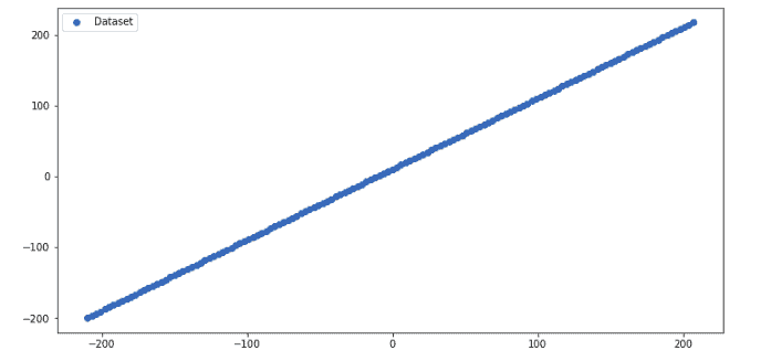
As you can see, the dataset is perfectly linear.
Splitting the dataset
Now, we will split the data into testing and training parts to evaluate the regression model’s performance after training.
# Splitting training and test data
X_train = X[:110]
y_train = y[:110]
X_test = X[110:]
y_test = y[110:]
# printing the input and output shapes
len(X_train), len(X_test)
Output:
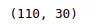
The output shows that there are 110 observations in the training part and 30 in the testing part.
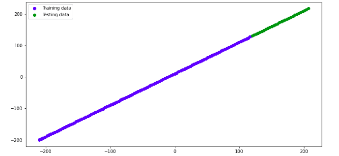
Let us visualize the dataset again to see how the testing and training datasets are distributed.
# size of the plot
plt.figure( figsize = (12,6))
# plotting training set and input data
plt.scatter(X_train, y_train, c='b', label = 'Training data')
plt.scatter(X_test, y_test, c='g', label='Test set')
plt.legend()
plt.show()
Output:
Defining the TensorFlow Regression model
Now, we can build the regression model with Neural Networks using TensorFlow step by step. Here we will create a straightforward regression model as a start to Neural Network Regression and visualize each step of building the Neural Network graphically to understand the TensorFlow implementation fully.
Let us first create the model. Here we will make the first layer ( the input layer) and specify the number of nodes to be one. Because in our dataset, the number of independent variables is one. So, the input layer should have one node to take the independent variable as an input. Also, we have one more dense layer, which specifies the output layer. We will also set the number of nodes in the output layer to one because, in the regression model, the output layer contains only one node.
# importing tensorflow module
import tensorflow as tf
# creating model and dense layer
model = tf.keras.Sequential([tf.keras.layers.InputLayer(
    input_shape=1),
    tf.keras.layers.Dense(1)])
The above code will create an input layer with only one node, as shown below:
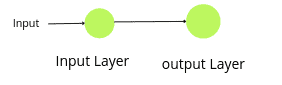
Now we are done with the first/input and output layers. Starting with the Neural Network, we will first create a simple neural network without hidden layers and train our model.
So, the next step is to compile the above-created input layer.
# compiling the neural network model
model.compile( loss = tf.keras.losses.mae,
              optimizer = tf.keras.optimizers.SGD(),#SGD-> stochastic gradient descent
              metrics = ['mae'])
As you can see, we have used Mean Absolute Error as the loss function. The loss function in Neural Network quantifies the difference between the excepted outcome and the outcome produced by the model.
The last step of building the model is to train the model on the training dataset. To train a model, we should specify the number of epochs. An epoch means training the neural network with all the training data for one cycle. In one epoch, we use all of the data exactly once. In other words, an epoch is an approach by which we pass the same dataset multiple times to the network to find optimal weights. A smaller number of epochs might lead to underfitting, while a larger number of epochs could lead to overfitting. So, we should choose epoch numbers that should be optimum or close to optimum.
So, we will start with fewer epochs to see how the number of epochs affects the predictions. Here, we will assign ten epochs to the training model, which means the model will iterate through the training dataset 10 times to find the best-fitted line/model.
# tensorflow run model/train model on input data
model.fit(tf.expand_dims(X_train, axis=-1), y_train), epochs=10)
Once the training is complete, we can use the testing dataset to evaluate the model’s performance. Notice that we have trained the model on ten epochs without any hidden layers.
Evaluating the model
Let us now use the testing dataset to predict the output values.
# Prediction of neural network model
preds = model.predict(X_test)
Let us now find the R-square score of the model.
#importing module
import sklearn
# Importing the required module
from sklearn.metrics import r2_score
# Evaluating the model
print('R score is :', r2_score(y_test, preds))
Output:

As you can see, the R-square score is negative, which shows the model has failed to follow the trend.
But it is always better to visualize the predictions to see how close they are to the actual values.
# size of the plot
plt.figure(figsize=(12,6))
# plots training data, test set and predictions
plt.scatter(X_train, y_train, c="b", label="Train data")
plt.scatter(X_test, y_test, c="g", label="Test set")
plt.scatter(X_test, preds, c="r", label="Predictions")
plt.legend()
plt.show()
Output:
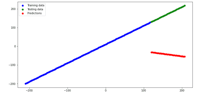
As you can see, the predictions are not even close to the actual values because the number of epochs was ten, and most probably, the model is under-fitted and failed to generalize the results. Let’s increase the number of epochs and train the same model ( without a hidden layer).
Increasing the epochs value
The last time we used a small number of epochs (10), our model could not train properly on the given dataset. We will increase the epoch value to 100 to see how the model will perform. Epoch value 100 means the model will iterate through the training dataset 100 times to find the best-fitted model.
# tensorflow run model/train model
model.fit(tf.expand_dims(X_train, axis=-1), y_train, epochs=100)
Now let us test the model using the testing dataset.
# Predictions
preds = model.predict(X_test)
The R-square score of the model with 100 epochs is:
# Importing the required module
from sklearn.metrics import r2_score
# Evaluating the model
print('R score is :', r2_score(y_test, preds))
Output:

As you can see, the model has failed to train properly, but at least we improved the predictions a little bit compared to last time.
We will also visualize the predictions.
# size of the plot
plt.figure(figsize=(12,6))
# plotting the garah
plt.scatter(X_train, y_train, c="b", label="Training data")
plt.scatter(X_test, y_test, c="g", label="Test set")
plt.scatter(X_test, preds, c="r", label="Predictions")
plt.legend()
plt.show()
Output:
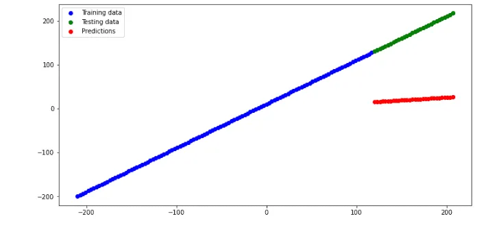
As you can see from the graph, the predictions are a little bit better than the previous, but still, the model is under-fitted.
We are getting under fitted model even after increasing the number of epochs because our neural network is incomplete. One of the main parts of the neural network is the hidden layer. And in the upcoming section, you will see how important is the hidden layer to building a better-performing deep learning model.
Adding a hidden layer with an activation function
At this time, we will add a new layer between the output and input layer, known as the hidden layer. Let us first understand how the hidden layer affects the model’s performance.
The capacity of a neural network model is defined by configuring the number of neurons (nodes) and the number of hidden layers. A model with less capacity may not be able to learn the training dataset sufficiently. In contrast, a model with too much capacity may memorize the training dataset, meaning it will overfit or get stuck or lost during the optimization process.
A model with a single hidden layer and a sufficient number of nodes can learn any mapping function. The number of layers in a model is referred to as its depth. Increasing the depth increases the model’s capacity, but we have to ensure that our model is not overfitted. So, we have to develop an optimum number of hidden layers and nodes in each layer.
Usually, one hidden layer with an optimum number of nodes can learn any mapping. So, now we will add one hidden layer to the model.
We will add a hidden layer of 10 nodes, apply the ReLU activation function on the dense layer, and see how the results will change.
# Model defining with 10 dense layers and rectified linear unit activation function
model = tf.keras.Sequential([tf.keras.layers.InputLayer(input_shape=1,),
  tf.keras.layers.Dense(10, activation = tf.keras.activations.relu),
  tf.keras.layers.Dense(1)
])
The above code will create a Neural Network that looks like this:
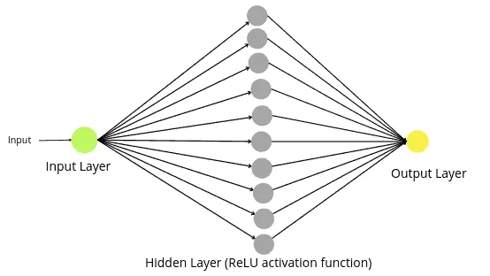
As you can see, now we have a fully built neural network with a hidden layer and expect better results.
Let us now compile and train the model on the training dataset.
# compiling the model
model.compile(loss=tf.keras.losses.mae,
                optimizer=tf.keras.optimizers.Adam(),
                metrics=['mae'])
# Training the model
model.fit(tf.expand_dims(X_train, axis=-1), y_train, epochs=100)
We will now use the testing data to make predictions and calculate the R-square score.
# Making pedictions
preds = model.predict(X_test)
# Evaluating the model
print('R score is :', r2_score(y_test, preds))
Output:

As you can see, this time, we got a really good score for the R-square, which means the model performed well.
Let us also visualize the predictions.
# size of the plot
plt.figure(figsize=(12,6))
# plotting the garah
plt.scatter(X_train, y_train, c="b", label="Training data")
plt.scatter(X_test, y_test, c="g", label="Test set")
plt.scatter(X_test, preds, c="r", label="Predictions")
plt.legend()
plt.show()
Output:
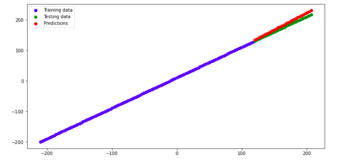
This plot shows that the predictions are close to the actual values, and we were able to build a neural regression model. So, based on what we have made so far, we can conclude that to build a neural regression model, we should:
- Create the input layer with one node.
- Create a hidden layer with optimum ( close to optimum nodes)
- Create an output layer with one node.
- Train the model on optimum ( close to optimum) epochs.
We have learned how to create and train a neural regression model, but how will we know how many nodes we should specify in the hidden layer and how many epochs will be best for the model? There are two methods to get the optimum number of nodes in the hidden layer and an optimum number of epochs.
- The first way is the try-and-error method. We can train the model on a different number of nodes and epoch values, as we did, and come up with the optimum number. But it is time-consuming.
- The second way is called parameter tuning, through which we can get optimum parameters for our model.
Using the parameter tuning method, let us learn how to find the optimum parameters for a neural regression model.
Finding optimum parameters using the parameter tuning method
We will use the parameter tunning method to find the optimum number of nodes in the hidden layer and an optimum number of epochs for the regression model.
In this section, we will use the Keras Tuner library that helps us to find optimal parameters for that TensorFlow model. So, first, let us import the required modules for the parameter tuning.
# importing required modules
from tensorflow import keras
import keras_tuner as kt
In the next step, we will define a user-defined function to create a neural regression model with maximum and minimum values for the nodes in the hidden layer.
# user define function
def model_builder(hp):

    # first layer of the model
    model = keras.Sequential([tf.keras.layers.InputLayer(input_shape=1,)])
    # specifying the min and max nodes for hidden layer
    hp_units = hp.Int('units', min_value=10, max_value=100)
    model.add(keras.layers.Dense(units=hp_units, activation='relu'))

    # output layer
    model.add(keras.layers.Dense(1))
    #compiling the model
    model.compile(optimizer=keras.optimizers.SGD(),
                    loss=tf.keras.losses.mae,
                    metrics=['mae'])
    return model
As you can see, the minimum number of nodes is ten, and the maximum is 100.
Now, we will initialize the tuner from the Keras Tunner library. It contains four different tuners: RandomSearch, Hyperband, BayesuabOptimization, and Sklearn. You can use any of them to find the optimum parameters for the model. In this tutorial, we will be using a Hyperband tuner that performs by random sampling and attempts to gain an edge by using time spent optimizing in the best way.
# initializing the tunner
tuner = kt.Hyperband(model_builder,
                     objective='val_loss',
                     max_epochs=200,
                    )
One of the important features of Keras is EarlyStopping. In Machine Learning, early stopping is a form of regularization used to avoid overfitting, and it stops the training of the model once a specified result is achieved. We will also use this Keras feature to ensure our model is not overfitted.
Let us initialize the EarlyStopping.
# Early stopping in keras
stop_early = tf.keras.callbacks.EarlyStopping(monitor='val_loss', patience = 4)
The patience parameter represents the number of epochs with no improvement after training is stopped.
First, let us search for the optimum number of nodes in the hidden layer by running the tunner.search() method.
# Seaching the tunner
tuner.search(X, y, validation_split=0.2, callbacks=[stop_early])
# Get the optimal hyperparameters
best_hps=tuner.get_best_hyperparameters(num_trials=1)[0]
# printing the optimal number of nodes
print('The optimal number of node in the hidden layer is: ', best_hps.get('units'))
Output:

As you can see that the tunner.search() method has found the optimum number of nodes in the hidden layer, 55.
Now, we will find the optimum number of epochs required to train the model without overfitting the model. We will use the optimum parameters that are returned by the tunner.search() method to train the model.
# creating model with the optimum parameters
model = tuner.hypermodel.build(best_hps)
# fixed max max epohcs to 300
Training_model = model.fit(X, y, epochs=300, validation_split=0.2)
# val_loss
val_acc_per_epoch = Training_model.history['val_loss']
# printing optimum eppoc
best_epoch = val_acc_per_epoch.index(max(val_acc_per_epoch)) + 1
print('Best epoch:',  best_epoch)
Output:

As you can see, our model’s optimum number of epochs is 170. We will again train the model using the optimum number of nodes and epochs.
Training regression model on optimum parameters
Again, let us create a Neural network with an input layer with one node, a hidden layer with 55 nodes, and an output with one node. We will fix the number of epochs to 170 for training.
# Creating modele complinin
model = tf.keras.Sequential([tf.keras.layers.InputLayer(
    input_shape=1,),
  tf.keras.layers.Dense(55, activation = tf.keras.activations.relu),
  tf.keras.layers.Dense(1)
])
# Complining the model
model.compile(loss=tf.keras.losses.mae,
                optimizer=tf.keras.optimizers.Adam(),
                metrics=['mae'])
# training the model on optimum epochs
model.fit(tf.expand_dims(X_train, axis=-1), y_train, epochs=170)
Once the training is complete, we can use the testing data to make predictions.
preds = model.predict(X_test)As we did before, let us find the R-square score of the model.
# Evaluating the model
print('R score is :', r2_score(y_test, preds))
Output:

We got an R-square of 0.94, which shows that our model has performed exceptionally well on the given dataset.
We will also visualize the predictions using a graph.
# size of the plot
plt.figure(figsize=(12,6))
# plotting the garah
plt.scatter(X_train, y_train, c="b", label="Training data")
plt.scatter(X_test, y_test, c="g", label="Testing data")
plt.scatter(X_test, preds, c="r", label="Predictions")
plt.legend()
plt.show()
Output:
As you can see, we have achieved excellent results by using the optimum nodes and epoch values.
Neural Network Regression model to predict House price
We have learned how to build a regression model using Neural Network. In this section, we will use the Neural Network regression model to predict the price of houses and see how the number of hidden layers affects the model’s performance. The dataset contains information about homes in Dushanbe city and their prices. You can access the dataset from this link.
Importing and exploring the dataset
Let us now use the Pandas module to import the dataset and print out a few rows.
# impprting the module
import pandas as pd
#importing regression data
House = pd.read_csv('Dushanbe_house.csv')
# heading
House.head()
Output:
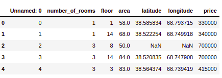
Let us remove the unnecessary column.
# dropping the column
House.drop('Unnamed: 0', axis=1, inplace=True)
As you can see, there are some null values in our dataset; we will also remove them.
# removing null avlues
House.dropna(inplace=True)
Now, let us check the shape of the dataset.
# input and output shapes
House.shape
Output:
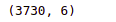
As you can see, there are 3730 houses in the dataset.
Splitting dataset
Now we will divide the dataset into dependent and independent variables.
# splitting our dataset into independent and dependent variables
x_data = House.drop('price', axis=1)
y_data = House.price
The next step is to split the dataset into testing and training parts.
# importing the module
from sklearn.model_selection import train_test_split
# splitting the dataset into test data and training set
X_train, X_test, y_train, y_test = train_test_split(x_data, y_data, test_size = 0.25, random_state = 0)
We have assigned 75% of the data to the training and the remaining 25% to the testing parts.
ANN regression with one hidden layer
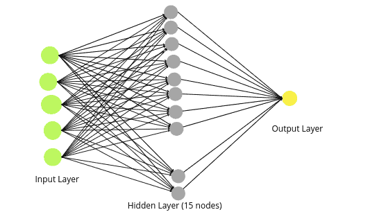
We will build a regression model to train on the training dataset. In the beginning, we will have a model with one hidden layer (15 nodes) and 100 epochs. We have selected nodes and epoch values randomly. You can use the tunning method (described above) to find the optimum values.
Also, we have five nodes in the input layer as the data has five input variables.
# fixing random state
tf.random.set_seed(42)
# building the model with hidden layer
model_house = tf.keras.Sequential([tf.keras.layers.InputLayer(
    input_shape=5,),
  tf.keras.layers.Dense(15, activation = tf.keras.activations.relu),
  tf.keras.layers.Dense(1)
])
# compiling the deep learning models , optimization function --> adam
model_house.compile(loss=tf.keras.losses.mae,
                optimizer=tf.keras.optimizers.Adam(),
                metrics=['mae'])
# Training data model
model_house.fit(X_train, y_train, epochs=100, verbose=0)
The above code will create the following Neural Network.
Once the training is complete, we can use the testing data to make predictions.
# making predictions on trained model
preds_house = model_house.predict(X_test)
We will now calculate the R-square score of the predictions.
# Importing the evaluation metrics
from sklearn.metrics import r2_score
# R-score --> evaluation metrics
print('R score is :', r2_score(y_test, preds_house))
Output:

The R-score shows that the model has failed to follow the trend.
Let us also visualize the actual and real values to see how the model has performed.
# fitting the size of the plot
plt.figure(figsize=(16, 8))
# plotting training and test
plt.plot([i for i in range(len(y_test))],y_test, label="actual values", c='r')
plt.plot([i for i in range(len(y_test))],preds_house, label="Predicted values", c='g')
# showing the plotting
plt.legend()
plt.show()
Output:
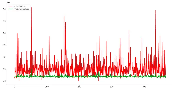
As you can see, the model has failed to perform well on the given dataset. Let’s keep all other parameters constant and add one more hidden layer to see how it will affect the model’s performance.
Training model with multiple hidden layers
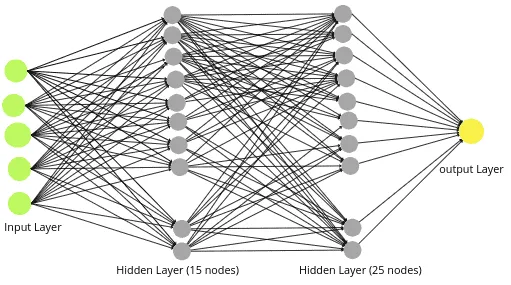
We will add one more hidden layer to the neural network, as our model failed to learn the trend with one hidden layer. We will add 25 nodes to the second hidden layer.
# fixing random state
tf.random.set_seed(42)
# building the model with hidden layer
model_house = tf.keras.Sequential([tf.keras.layers.InputLayer(
    input_shape=5,),
  tf.keras.layers.Dense(15, activation = tf.keras.activations.relu),
  tf.keras.layers.Dense(25, activation = tf.keras.activations.relu),

  tf.keras.layers.Dense(1)
])
# compiling the model
model_house.compile(loss=tf.keras.losses.mae,
                optimizer=tf.keras.optimizers.Adam(),
                metrics=['mae'])
# Training the model
model_house.fit(X_train, y_train, epochs=100, verbose=0)
The above code will create the following neural network:
We will test the model on the testing dataset and find the R-square score.
# Evaluating the model
print('R score is :', r2_score(y_test, preds_house))
Output:

This time, we got a pretty good R-square score, which means our model performed better. We will also visualize the predictions and actual values.
# fitting the size of the plot
plt.figure(figsize=(16, 8))
# plotting the graphs
plt.plot([i for i in range(len(y_test))],y_test, label="actual values", c='r')
plt.plot([i for i in range(len(y_test))],preds_house, label="Predicted values", c='g')
# showing the plotting
plt.legend()
plt.show()
Output:
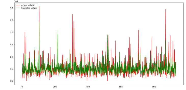
As you can see, the predictions are close to the actual values when we trained the model on two hidden layers. So, an increasing number of hidden layers increases the model’s performance but ensures that our model is not overfitted.
You can also use the parameter tunning method to find the optimum parameters, as we did before, to find the optimum number of nodes and epochs.
Summary
Neural network regression is an ML algorithm used to predict continuous values. Unlike traditional regression methods, which typically require a large amount of data to produce accurate predictions, neural network regression can learn from small datasets and still produce reliable results. In addition, neural networks can handle non-linear relationships between variables, making them well-suited for modeling complex real-world phenomena. TensorFlow, an open-source software library for Machine Learning, offers a robust framework for implementing neural network regression models. In this article, we learned about Neural Network regression in detail. We learned how to build a regression model using TensorFlow and implement it on a real dataset.
