Getting started with the Extra Trees algorithm in Python

An extra tree is an algorithm used for classification and regression tasks. It works by randomly selecting a subset of features and then training a Decision Tree on them. The tree is then pruned only to contain the most important features for making predictions. The Extra tree algorithm is considered an efficient and accurate machine learning method. It has outperformed other popular methods such as support vector machines and random forests. This article will discuss how the Extra Tree algorithm works and how it differs from the Random forest algorithm. We will also implement it on regression and classification datasets using Python.

Before going into the Extra Trees algorithm, make sure you have a solid knowledge of the Decision Trees and Random Forest algorithm because the Extra Trees algorithm uses those algorithms with slight changes.

What is the Extra Trees algorithm?

The extra tree, also known as the Extreme Randomized Tree, generates predictive models for classification and regression problems. It is similar to other methods such as decision trees and random forests, but it uses extra information about the data to improve predictive accuracy. Additionally, the extra tree algorithm is faster and easier to implement than other methods. As a result, it is a powerful tool for data mining and predictive modeling.

Difference between Extra tree and Random forest

Extremely Randomized Tree is an ensemble learning technique aggregating the results of multiple de-correlated decision trees collected in a forest to output. It is very similar to a Random Forest, and the only difference is in the construction of the decision trees.

The main difference between the Random Forest and Extra tree algorithm are as follows:

• Random Forest uses bootstrap replicas; it subsamples the input data with replacement, whereas Extra Trees uses the original dataset.
• Another difference is the selection of cut points to split nodes. Random Forest chooses the optimum split, while Extra Trees chooses it randomly. However, once the split points are selected, the two algorithms determine the best one between all the subsets of features. Therefore, Extra Trees adds randomization but still has optimization.

Advantages of Extra trees algorithm

The following are some of the advantages of the extra trees algorithm

• As we discussed, it uses the original sample instead of a bootstrap replica, reducing bias.
• Also, the highly randomized tree algorithm randomly chooses each node’s split point, which reduces variance.
• It is much faster than the decision tree and random forest algorithm as it does not spend time choosing the optimum split point.
• As the algorithm reduces bias and variance, there are significantly fewer chances of the model being overfitted or underfitting.

Implementation of Extra Trees regressor using Python

Let us jump into the implementation part and apply the Extra trees regressor on a regression dataset. In this section, we will use a WHO dataset about the life expectancy of various countries. You can read more about the input and output variables of the dataset from this link.

Before going to the implementation part, ensure that you have installed the following modules on your system.

• sklearn
• pandas
• NumPy
• matplotlib
• seaborn

You can install these modules by running the following commands in the cell of the Jupyter notebook.

%pip install skearn
pip install pandas
pip install numpy
pip install matplotlib
pip install searbonr

Once the required modules are installed successfully, we can go to the implementation part.

Importing and exploring the dataset

We will use the Pandas DataFrame to import and process the dataset:

# importing the module
import pandas as pd
# importig the dataset
dataset = pd.read_csv("Life Expectancy Data.csv")
# head method
dataset.head()

Output:

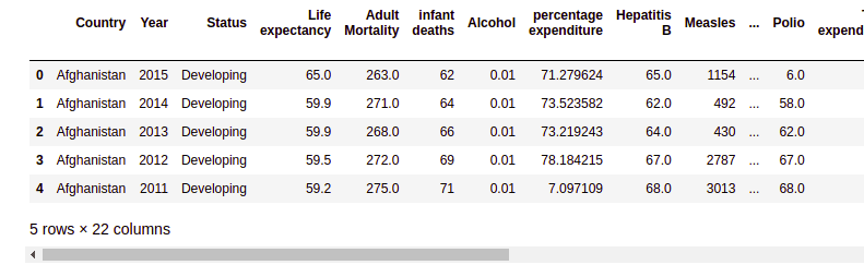
Notice that there is a total of 22 columns. In this article, we will take the life expectancy column as our target variable and use the Extra Trees algorithm to predict life expectancy.

Let us use the info() method to get more information about the dataset.

# info method
dataset.info()

Output:

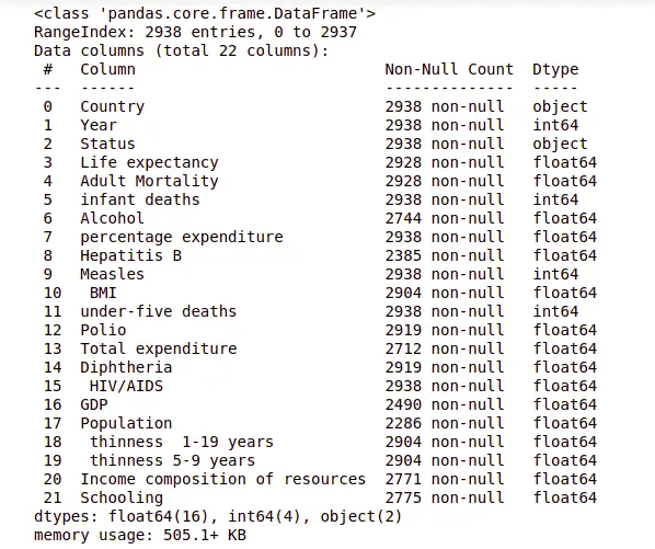
The information shows that the total number of observations is 2938 and except for two columns, all others are either floating or integer values.

Let us now find the correlation matrix to see if some columns are strongly co-related; we will remove them.

# importing the required modules
import seaborn as sns
import numpy as np
import matplotlib.pyplot as plt
# setting the size of the figure
f, ax = plt.subplots(figsize=(10, 8))
# finding the correlation
corr = dataset.corr()
# plotting the correlation
sns.heatmap(corr, mask=np.zeros_like(corr, dtype=np.bool), cmap=sns.diverging_palette(220, 10, as_cmap=True),
            square=True, ax=ax)

Output:

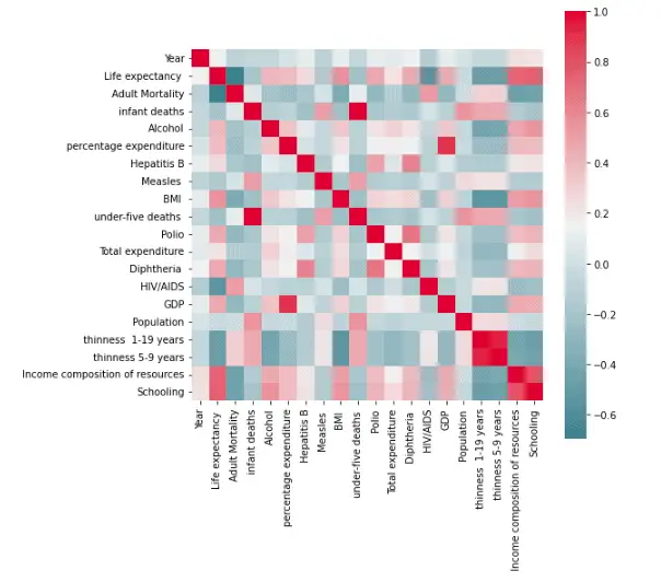
As you can see, some of the input data are strongly correlated, such as infant deaths and under-five deaths, GDP, and percentage expenditure. So, we will drop any of them.

# dropping the correlated columns
dataset.drop('GDP', axis= 1, inplace=True)
dataset.drop('infant deaths', axis=1, inplace=True)

Now let us visualize a few dataset columns to get more information. First, we will visualize the life expectancy of developing and developed countries based on alcohol consumption.

# ploting graph
alcohol_life_exp = sns.scatterplot(data=dataset, x="Alcohol", y="Life expectancy ", hue="Status")
alcohol_life_exp

Output:

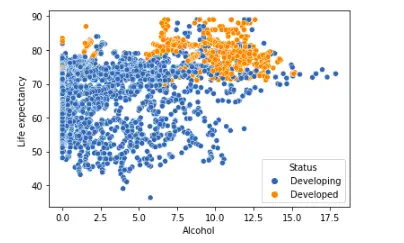
The above plot shows that developed countries have more life expectancy than developing countries.

Let us also plot the schooling and life expectancy for the developing and developed countries.

# ploting grapp
alcohol_life_exp = sns.scatterplot(data=dataset, x="Schooling", y="Life expectancy ", hue="Status")
alcohol_life_exp

Output:

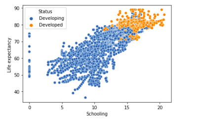
As you can see, there is a clear difference between schooling in developed countries and developing countries.

The last step of data processing is to see if there are any null values.

# calculating the null values
dataset.isnull().sum()

Output:

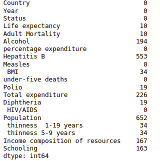
Notice that there are many null values, so that we will remove them from the dataset.

# removing the null values
dataset.dropna(axis=0, inplace=True)

Once we remove null values, we can proceed to the next step.

Splitting the dataset

Before splitting the dataset, we need to convert the categorical/object values to numeric values to train the model.

# Import label encoder
from sklearn import preprocessing
  
# label_encoder object knows how to understand word labels.
label_encoder = preprocessing.LabelEncoder()
  
# Encode labels in column 'species'.
dataset['Country']= label_encoder.fit_transform(dataset['Country'])
dataset['Status']= label_encoder.fit_transform(dataset['Status'])

Once the encoding is complete, we can divide the dataset into inputs and outputs.

# Splitting the dataset
Inputs = dataset.drop('Life expectancy ', axis=1)
output = dataset['Life expectancy ']

Now we can divide the dataset into training and testing datasets.

# importing the module
from sklearn.model_selection import train_test_split
# splitting the dataset 
X_train, X_test, y_train, y_test=train_test_split(Inputs, output, test_size=0.25)

Notice that we assigned 25% of the data to the testing and 75% to the training.

Training and testing the Extra Tree regressor

Let us import the required model and train it using the training dataset.

# importing the module
from sklearn.ensemble import ExtraTreesRegressor
# initializing the model
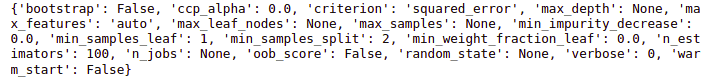
ET_regressor = ExtraTreesRegressor()

Notice that we have used all default parameters. We can check the values of default parameters by printing the model’s parameters.

# printing the parameters
print(ET_regressor.get_params())

Output:

Let us now train the model using the training dataset.

# Training the model
ET_regressor.fit(X_train, y_train)

Now, we will use the testing data to make predictions.

# Making predictions
Regressor_pred = ET_regressor.predict(X_test)

We will use different strategies to see how well the model makes predictions.

Visualizing the results

Let us visualize the actual and predicted values to see how well the model made predictions.

# fitting the size of the plot
plt.figure(figsize=(15, 8))
# plotting the graphs
plt.plot([i for i in range(len(y_test))],y_test, color = 'green',label="actual values")
plt.plot([i for i in range(len(y_test))],Regressor_pred, color='red', label="Predicted values")
# showing the plotting
plt.legend()
plt.show()

Output:

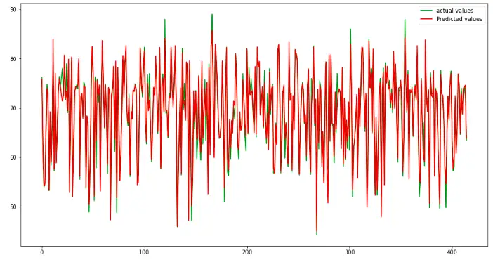
The red lines show the predicted values, and the green shows the actual values. Let us also calculate the R-square value of the model.

# Importing the required module
from sklearn.metrics import  r2_score
# Evaluating model performance
print('R-square score is :', r2_score(y_test, Regressor_pred))

Output:

As you can see, we get a good R-square which means our model has performed well.

Extreme Randomized Tree vs. Decision Tree algorithm

Now let us use the same dataset to train the Decision tree and compare the results.

# import decision tree
from sklearn.tree import DecisionTreeRegressor
# instantiate the regressor
decision_tree = DecisionTreeRegressor()
# fit the model
decision_tree.fit(X_train, y_train)

We will now make predictions using the testing dataset.

# testing the model
y_pred = classifier.predict(X_test)

Once the predictions are complete, we can evaluate the results using the R-square score.

# Evaluating model performance
print('R-square score is :', r2_score(y_test, y_pred))

Output:

Notice that the R-square score of the Decision Tree is less than the R-square score of the Extra Trees regressor, which means the Extra Trees regressor performed well on the given dataset, the Decision Tree Regressor.

Implementation of Extra Trees Classifier using Python

Now we will apply the Extra Trees classifier to a classification dataset. We will use the handwritten digits recognition dataset from the submodule of sklearn. The dataset contains the different pixel values for each digit, which you can download using this link.

Importing and exploring the dataset

Let us now load the dataset and print out a few rows to get familiar with the dataset.

# importing module
from sklearn import datasets
# loading dataset
digits = datasets.load_digits()
# convertig the dataset into pandas dataframe
digit = pd.DataFrame(digits.data, columns=digits.feature_names)
# printing rows
digit.head()

Output:

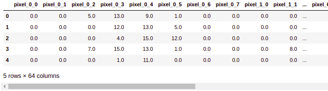
The columns contain the pixel values for each of the digits.

We know that the pixel values combine to make an image. Let us now visualize any of the digits from the dataset.

# importing the module
import matplotlib.pyplot as plt
# printing the image of 1
plt.imshow(digits.images[1], cmap=plt.cm.gray_r, interpolation='nearest')
plt.show()

Output:

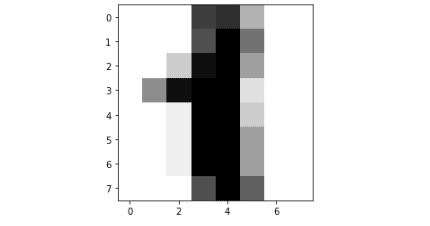
You can see that we have visualized digit 1.

Training and testing the classifier

Now we will divide the dataset into input values and output values.

# splitting the data into inputs and outputs
Input, output = datasets.load_digits(return_X_y=True)

The next step is to split the dataset into testing and training parts so that after training the model, we can use the testing data to evaluate it.

# importing the module
from sklearn.model_selection import train_test_split
# splitting the dataset
X_train, X_test, y_train, y_test = train_test_split(Input, output, test_size=0.25)

As you can we, we have assigned 25% of the data for testing and 75% for the training.

Now, we will load the classifier and train the model.

# importing the module
from sklearn.ensemble import ExtraTreesClassifier
# initializing the model
ET_classifier = ExtraTreesClassifier()
# Training the model
ET_classifier.fit(X_train, y_train)

Once the training is complete, we can use the testing dataset to make predictions.

# making predictions
classifier_pred = ET_classifier.predict(X_test)

We will use different classification evaluation matrices to evaluate the performance.

Evaluating the classifier

A confusion matrix is a tool for predictive analysis in machine learning, especially for the classification model. We will use the confusion matrix to see how well our model was in predicting the testing dataset.

# importing seaborn
import seaborn as sns
# Making the Confusion Matrix
from sklearn.metrics import confusion_matrix
# providing actual and predicted values
cm = confusion_matrix(y_test, classifier_pred)
# If True, write the data value in each cell
sns.heatmap(cm,annot=True)

Output:

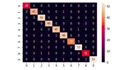
The above graph shows that our model has performed exceptionally well and was able to classify most of the testing data points correctly.

Now let us also find the accuracy of the model.

# importing accuracy score
from sklearn.metrics import accuracy_score
#accuracy score
accuracy_score(y_test,y_pred)

Output:

The output shows that our model correctly classified 98% of the input data.

Random Forest Classifier Vs. Extra Tree Classifier

Now let us train the Random forest classifier model on the same dataset and compare the results. First, we will import the Random forest classifier and train it using the training data.

# import Random Forest classifier
from sklearn.ensemble import RandomForestClassifier
# instantiate the classifier 
classifier = RandomForestClassifier()
# fit the model
classifier.fit(X_train, y_train)

Once the training is complete, we can use the testing data to make predictions.

# testing the model
y_pred = classifier.predict(X_test)

Let us also use a confusion matrix to visualize the results of the Random Forest classifier.

# providing actual and predicted values
cm = confusion_matrix(y_test, y_pred)
# If True, write the data value in each cell
sns.heatmap(cm,annot=True)

Output:

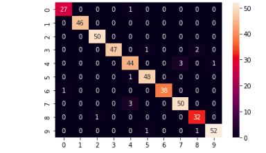
The confusion matrix shows that the Random Forest classifier had also performed well and correctly classified most of the digits.

Now we will find the accuracy of the model.

# printing the accuracy of the model
print(accuracy_score(y_test, y_pred))

Output:

The above output shows that the model has correctly classified 96% of the data points; however, it is slightly less than the Extra tree classifier.

Summary

Extremely Randomized Trees, also known as Extra Trees for short, is an ensemble machine learning algorithm. You can use it for both classification and regression modeling. It is similar to a Random forest with a slight change in splitting the nodes in the decision tree. This article covered how the Extra Trees algorithm differs from the Random forest algorithm. We also implement the algorithm on classification and regression datasets.