Naive Bayes Classifier Python Tutorial

Naive Bayes is a statistical classification technique based on the Bayes Theorem and one of the simplest Supervised Learning algorithms. This Naive Bayes Classifier Python tutorial will help you to get quick, accurate, and trustworthy results for large datasets. This article will discuss the theory of Naive Bayes classification and its implementation using Python.

A Naive Bayes classifier assumes that the effect of a particular feature in a class is independent of other features and is based on Bayes’ theorem. Bayes’ theorem is a mathematical equation used in probability and statistics to calculate conditional probability. In other words, you can use this theorem to calculate the probability of an event with functions like the Gaussian Probability Density function based on its association with another event.

The simple formula of the Bayes theorem is:

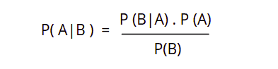
Where P(A) and P(B) are two independent events and (B) is not equal to zero.

• P(A | B): is the conditional probability of an event A occurring given that B is true.
• P( B | A): is the conditional probability of an event B occurring given that A is true.
• P(A) and P(B):  are the probabilities of A and B occurring independently of one another (the marginal probability).

What is Naive Bayes Classification?

The Naive Bayes classification algorithm is a probabilistic classifier and belongs to Supervised Learning. It is based on probability models that incorporate strong independence assumptions. The independence assumptions of the Naive Bayes models often do not impact reality. Therefore they are considered naive.

Another assumption made by the Naive Bayes classifier is that all the predictors have an equal effect on the outcome. The Naive Bayes classification has the following different types:

• The Multinomial Naive Bayes method is a common Bayesian learning approach in natural language processing. Using the Bayes theorem, the program estimates the tag of a text, such as an email or a newspaper piece. It assesses the likelihood of each tag of multinomial Naive Bayes for a given sample and returns the tag with the highest possibility.
• The Bernoulli Naive Bayes is a part of the family of Naive Bayes. It only takes binary values. Multiple features may exist, but each is assumed to be a binary-valued (Bernoulli, boolean) variable. Therefore, this class requires samples to be represented as binary-valued feature vectors.
• The Gaussian Naive Bayes is a variant of Naive Bayes that follows Gaussian normal distribution and supports continuous data. To build a simple model using Gaussian Naive Bayes, we assume the data is characterized by a Gaussian distribution with no covariance (independent dimensions) between the parameters. This model may fit by applying the Bayes theorem to calculate the mean and standard deviation of the points within each label.

The Naive Bayes classifier makes two fundamental assumptions on the observations.

• The target classes are independent of each other. Consider a rainy day with strong winds and high humidity. A Naive classifier would treat these two features, wind and humidity, as independent parameters. That is to say, each feature would impose its probabilities on the outcome, such as rain in this case.
• Prior probabilities for the target classes are equal. That is, before calculating the posterior probability of each class, the classifier will assign each target class the same prior probability.

When to use the Naive Bayes Classifier?

Naive Bayes classifiers tend to perform especially well in any of the following situations:

• When the naive assumptions match the data.
• For very well-separated categories, when model complexity is less important.
• And for very high-dimensional data, when model complexity is again less important.

The last two points appear unrelated, but they are related to each other. As a dataset’s dimension grows, it becomes less likely that any two points will be discovered nearby. This means that clusters in high dimensions tend to be more separated than clusters in low dimensions,

The Naive Bayes classifier has the following advantages.

• Naive Bayes classification is extremely fast for training and prediction especially using logistic regression.
• It provides straightforward probabilistic prediction.
• Naive Bayes has a very low computation cost.
• It can efficiently work on a large dataset.
• It performs well in the case of discrete response variables compared to continuous variables.
• It can be used with multiple class prediction problems.
• It also performs well in the case of text analytics problems.
• When the assumption of independence holds, a Naive Bayes classifier performs better than other models like Logistic Regression.

Real-life applications using Naive Bayes Classification

The Naive Bayes algorithm offers plenty of advantages to its users. That’s why it has a lot of applications in various industries, including Health, Technology, Environment, etc. Here are a few of the applications of the Naive Bayes classification:

• It is used in text classification. For example, News on the web is rapidly growing, and each news site has its different layout and categorization for grouping news. To achieve better classification results, we apply the naive Bayes classifier to classify news content based on news code.
• Another application of Naive Bayes classification is Spam filtering. It typically uses a bag of words features to identify spam e-mails. Naive Bayes classifiers work by correlating the use of tokens (typically words or sometimes other things), with spam and non-spam e-mails and then using Bayes’ theorem to calculate the probability that an email is or is not spam.
• One of the advantages of the Naive Bayes Classifier is that it takes all the available information or data point to explain the decision. When dealing with medical data, the Naïve Bayes classifier considers evidence from many attributes to make the final prediction of the class label and provides transparent explanations of its decisions. That is why it has many applications in the health sector as well.
• Weather prediction has been a challenging problem in the meteorological department for years. Even after technological and scientific advancements, the accuracy in weather prediction has never been sufficient. However, Naive Bayes classifiers give high-accuracy results when predicting weather conditions.
• Its assumption of feature independence, and its effectiveness in solving multi-class problems, make it perfect for performing Sentiment Analysis. Sentiment Analysis identifies a target group’s positive or negative sentiments.
• Collaborative Filtering and the Naive Bayes algorithm work together to build recommendation systems. These systems use data mining and Machine Learning to predict whether the user would like a particular resource. 

Mathematical calculations behind Naive Bayes Classification

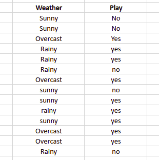
Let’ u’s calculate the event occurring/classifying using the Naive Bayes classification method to calculate probabilities by taking a simple example. Given an example of weather conditions and playing sports, we need to calculate the probability of playing sports and not playing sports, finding out whether the statement has dependent or independent variables. And classify using different classification algorithms whether players will play or not depending on the weather condition. The sample data set is as follows:

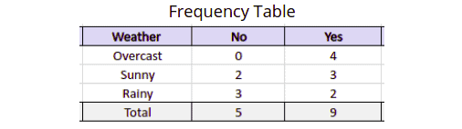
You can use the above example’s given data set frequency and likelihood tables to simplify prior and posterior probability calculations. The Frequency table shows how often labels appear for each feature. These tables will assist us in calculating the prior and posterior probabilities. 

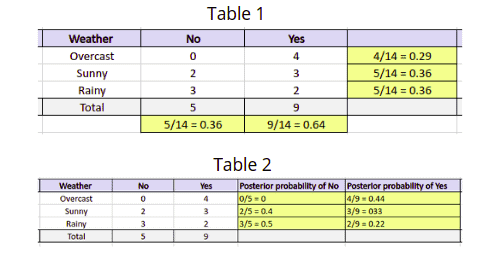
Now let us divide the above frequency table into prior and posterior probabilities. The prior probability is the probability of an event before new data is collected. In contrast, the posterior probability is the statistical probability that calculates the hypothesis to be true in the light of relevant observations.

Table 1 shows the prior probabilities of labels, and Table 2 shows the posterior probability.

Once our model has the above data, it can easily classify any testing/input value. For example, you want to calculate the probability of playing when the weather is overcast. We can calculate the following calculations to predict whether a player will play.

Probability of Playing:

We have the formula for the Naive Bayes classification, which is

P(Yes | Overcast) = P(Overcast | Yes) P(Yes) / P (Overcast).

Now, let’s calculate the prior probabilities:

P(Overcast) = 4/14 = 0.29

P(Yes)= 9/14 = 0.64

The next step is to find the posterior probability, which can be easily calculated by:

P(Overcast | Yes) = 4/9 = 0.44

Once we have the posterior and prior probabilities, we can put them back in our main formula to calculate the probability of playing when the weather is overcast.

P(Yes | Overcast) = 0.44 * 0.64 / 0.29 = 0.98

Probability of Not Playing:

Similarly, we can calculate the probability of not playing any sports when overcast weather.

First, let us calculate the prior probabilities.

P(Overcast) = 4/14 = 0.29

P(No)= 5/14 = 0.36

The next step is to calculate the posterior probability, which is:

P(Overcast | No) = 0/9 = 0

By putting these probabilities in the main formula, we get:

P(No | Overcast) = 0 * 0.36 / 0.29 = 0

We can see that the probability of a Playing class is higher, so if the weather is Overcast players will play sports.

Naive Bayes Classifier Python Implementation

Let’s implement the Naive Bayes Classification using the sklearn module. We will use a sample data set, which you can download here. This simple data set contains only two output classes (binary classification dataset). The input values contain the age and salary of a person, and the output class contains whether the person purchased the product or not.

Importing and defining Binary Dataset for Naive Bayes Classification

We will use the following modules to implement Naive Bayes classification using Python. You can install them using the pip command on your system.

# importing the libraries
import numpy as np
import matplotlib.pyplot as plt
import pandas as pd
import seaborn as sns

Once we have imported all the required modules, the next step is to import the data set and split the data sets into inputs and outputs. You can get access to the data set from this link.

# importing the dataset
dataset = pd.read_csv('NaiveBayes.csv')
# split the data into inputs and outputs
X = dataset.iloc[:, [0,1]].values
y = dataset.iloc[:, 2].values

The next step is to divide the input and output values into the training and testing part so that once the model’s training is complete, we can evaluate its performance using testing data.

# training and testing data
from sklearn.model_selection import train_test_split
# assign test data size 25%
X_train, X_test, y_train, y_test =train_test_split(X,y,test_size= 0.25, random_state=0)

We set test_size=0.25, which means 25% of the whole data set will be assigned to the testing part, and the remaining 75% will be used for the model’s training.

The next step is to scale our dataset to be ready to be used for the training.

# importing standard scaler
from sklearn.preprocessing import StandardScaler
# scalling the input data
sc_X = StandardScaler() 
X_train = sc_X.fit_transform(X_train)
X_test = sc_X.fit_transform(X_test)

Note: scaling (or standardization) of a dataset is a common requirement for many machine learning estimators: they might misbehave if the individual features do not more or less look like standard normally distributed data.

Training the model using Bernoulli Naive Bayes classifier

We’ll use the Bernoulli Naive Bayes classifier in this article section to train our model.

# importing classifier
from sklearn.naive_bayes import BernoulliNB
# initializaing the NB
classifer = BernoulliNB()
# training the model
classifer.fit(X_train, y_train)
# testing the model
y_pred = classifer.predict(X_test)

Now let us check the accuracy of the predicted values using the Bernoulli Naive Bayes classifier.

# importing accuracy score
from sklearn.metrics import accuracy_score
# printing the accuracy of the model
print(accuracy_score(y_pred, y_test))

Output:

We got an accuracy of 80% when we trained our model using Bernoulli Naive Bayes classifier.

Training model using Gaussian Naive Bayes Classifier

Now, let’s train our model using the Gaussian Naive Bayes classifier (a type of Naive Bayes Classifier).

# import Gaussian Naive Bayes classifier
from sklearn.naive_bayes import GaussianNB
# create a Gaussian Classifier
classifer1 = GaussianNB()
# training the model
classifer1.fit(X_train, y_train)
# testing the model
y_pred1 = classifer1.predict(X_test)

Let’s check the accuracy of our model:

# importing accuracy score
from sklearn.metrics import accuracy_score
# printing the accuracy of the model
print(accuracy_score(y_test,y_pred1))

Output:

This time we got an accuracy of 91% when we trained the model on the same dataset.

Evaluating Naive Bayes Classification performance

This article’s part will demonstrate how to evaluate the performance of the Naive Bayes classification model.

Confusion Matrix for Binary classification

The confusion matrix is also known as the error matrix. It is a table layout that allows visualization of the performance of a classification algorithm. Each row of the matrix represents the instances in an actual class of a class variable. In contrast, each column represents the instances in a predicted class with class probabilities or vice versa.

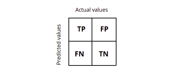
The confusion matrix for binary classification is a 2×2 matrix representing the actual and predicted values. It helps us calculate accuracy, precision, recall, and f1-score, which helps us evaluate the model’s performance.

Evaluation of Bernoulli Naive Bayes classifier

Let’s evaluate ourBernoulli Naive Bayes model using a confusion matrix that will visually help us see the number of correct and incorrect classified classes. First of all, we’ll visualize our model’s results. The predicted values are stored in a variable named y_pred, the target variable.

# importing the required modules
import seaborn as sns
from sklearn.metrics import confusion_matrix
# passing actual and predicted values
cm = confusion_matrix(y_test, y_pred)
# true write data values in each cell of the matrix
sns.heatmap(cm, annot=True)
plt.savefig('confusion.png')

Output:

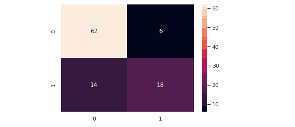
The confusion matrix helps us know which class has been mispredicted.

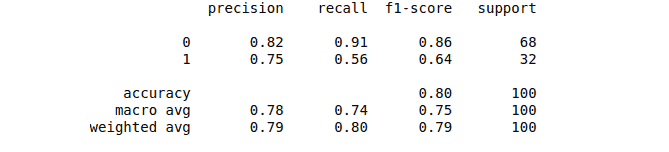
We can also print the classification report, which will help us further evaluate our model’s performance.

# importing classification report
from sklearn.metrics import classification_report
# printing the report
print(classification_report(y_test, y_pred))

Output:

Evaluation of Gaussian Naive Bayes Classifier

Let’s evaluate theGaussian Naive Bayes model. The predicted values are stored in a variable named y_pred1.

# importing the required modules
import seaborn as sns
from sklearn.metrics import confusion_matrix
# passing actual and predicted values
cm = confusion_matrix(y_test, y_pred1)
# true write data values in each cell of the matrix
sns.heatmap(cm,annot=True)
plt.savefig('confusion.png')

Output:

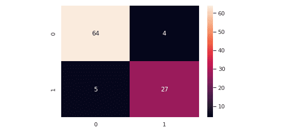
Note: the Gaussian naive Bayes classifier performed very well on this dataset, as shown in the confusion matrix. Let us now print out the classification report as well,

# importing classification report
from sklearn.metrics import classification_report
# printing the report
print(classification_report(y_test, y_pred1))

Output:

Features Encoding

In real life, the data does not always consist of numeric values. For example, playing or not playing are not numeric values. In such scenarios, we need to convert the non-numeric data to numeric values before feeding data to our model. For example, we have the following dataset about whether players will play sports or not, depending on the weather and temperature.

# assigning features and label variables
weather = ['Sunny','Sunny','Overcast','Rainy','Rainy','Rainy','Overcast','Sunny','Sunny', 'Rainy','Sunny','Overcast','Overcast','Rainy']
# output class
play = ['No','No','Yes','Yes','Yes','No','Yes','No','Yes','Yes','Yes','Yes','Yes','No']

Note: the input and output are not numeric values. Before feeding this data to our model, we have to encode the non-numeric values into numeric ones. for example, Overcast = 0, Rainy = 1, Sunny = 2. This is called label encoding.

# Import LabelEncoder
from sklearn import preprocessing
# creating LabelEncoder
labelCode = preprocessing.LabelEncoder()
# Converting string labels into numbers.
wheather_encoded=labelCode.fit_transform(weather)

The LabelEncoder will convert the string values to numeric values. For example, if we print the encoded weather, it will no longer contain numeric values.

print(weather_encoded)

Output:

Similarly, we can also encode the play class.

# import LabelEncoder
from sklearn import preprocessing
# creating LabelEncoder
labelCode = preprocessing.LabelEncoder()
# converting string labels into numbers.
label=labelCode.fit_transform(play)

Generating model

We have already seen that our input values are in a single-dimensional array. By default, the model training takes values in multi-dimensional arrays. We will get the following error if we feed the data without further changes.

# import Gaussian Naive Bayes model
from sklearn.naive_bayes import GaussianNB
# create a Gaussian Classifier
model = GaussianNB()
# train the model using the training sets
model.fit(weather_encoded, label)

Output:

So, we need to convert our data to the 2D array before feeding it to our model. Here we will use NumPy array and reshape() method to create a 2D array.

# importing numpy module
import numpy as np
# converting 1D array to 2D
weather_2d = np.reshape(weather_encoded, (-1, 1))

Now our data is ready. We can train our model using this data.

# import Gaussian Naive Bayes model
from sklearn.naive_bayes import GaussianNB
# create a Gaussian Classifier
model = GaussianNB()
# train the model using the training sets
model.fit(weather_2d, label)

We used the Gaussian Naive Bayes classifier to train our model. Let us predict the output by providing a testing input.

# predicting the odel
predicted= model.predict([[0]]) # 0:Overcast
# printing predicted value
print(predicted)

Output:

The output value 1 indicates that players will Play when there’s an Overcast weather.

Naive Bayes Classification with Multiple Labels

Up to this point, we have learned Naive Bayes classification with binary labels. This section will teach about Naive Bayes classification for multiple labels. For example, if we want to categorize a news story regarding technology, entertainment, politics, or sports.

For the training, we will use the built-in data set from the sklearn module named load_wine. This dataset results from a chemical analysis of wines grown in the same region in Italy but derived from three different cultivars.

The dataset consists of 13 features (alcohol, malic_acid, ash, alcalinity_of_ash, magnesium, total_phenols, flavanoids, nonflavanoid_phenols, proanthocyanins, color_intensity, hue, od280/od315_of_diluted_wines, proline) and type of wine cultivar. This data has three types of wine Class_0, Class_1, and Class_3. We can build a model to classify the type of wine using the Naive Bayes Classification.

Loading and Exploring the dataset

First, we need to import datasets from the sklearn module and load the load_wine().

# import scikit-learn dataset library
from sklearn import datasets
# load dataset
dataset = datasets.load_wine()

Next, we can print the input/features and target/output variables’ names to ensure the desired dataset.

# print the names of the 13 features
print ("Inputs: ", dataset.feature_names)
# print the label type of wine
print ("Outputs: ", dataset.target_names)

Output:

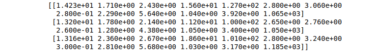
We check the type of data (numeric/non-numeric) by printing three rows from the dataset.

# print the wine data features
print(dataset.data[0:3])

Output:

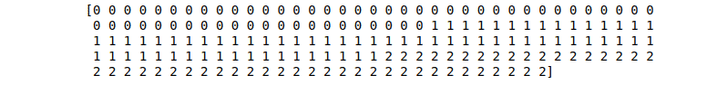
We can also check the output values to verify that it is a multi-class classification dataset.

# print the wine labels 
print(dataset.target)

Output:

Training the model using multiclass labels

Before feeding the dataset to our model, let us split the dataset into training and testing parts to evaluate our model by providing the testing dataset.

# import train_test_split function
from sklearn.model_selection import train_test_split
# input and outputs
inputs = dataset.data
outputs = dataset.target
# split dataset into training set and test set
X_train, X_test, y_train, y_test = train_test_split(inputs, outputs, test_size=0.3, random_state=1)

Once the splitting is complete, we can feed our model with the training data.

# import Gaussian Naive Bayes model
from sklearn.naive_bayes import GaussianNB
# create a Gaussian Classifier
classifer = GaussianNB()
# train the model using the training sets
classifer.fit(X_train, y_train)
# predict the response for test dataset
y_pred = classifer.predict(X_test)

Note: we have used the Gaussian Naive Bayes classification method for the training.

Let us now check the accuracy of our model:

# import scikit-learn metrics module for accuracy calculation
from sklearn import metrics
# printing accuracy
print("Accuracy:", metrics.accuracy_score(y_test, y_pred))

Output:

We got 98% accurate results, which is pretty high accuracy.

Evaluation of Naive Bayes Classifier for multi-classification

The Confusion Matrix is not only used to evaluate binary classification. It can also help evaluate multiclass-classification problems as well. The number of columns/rows will equal the number of output classes.

Let’s evaluate our model, which was trained by multi-labeled data using a confusion matrix.

# importing the required modules
import seaborn as sns
from sklearn.metrics import confusion_matrix
# passing actual and predicted values
cm = confusion_matrix(y_test, y_pred)
# true Write data values in each cell of the matrix
sns.heatmap(cm, annot=True)
plt.savefig('confusion.png')

Output:

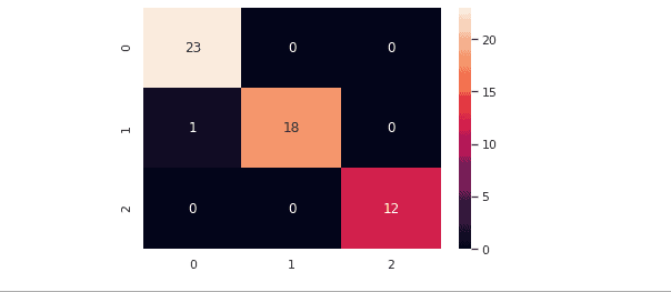
Note: there were three labels in our dataset, as shown in the confusion matrix.

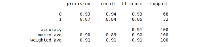
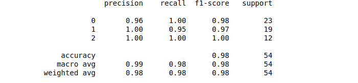
Let us now print out the classification score for our model.

# Importing classification report
from sklearn.metrics import classification_report
# printing the report
print(classification_report(y_test, y_pred))

Output:

Naive Bayes Classification using sklearn and AWS SageMaker Studio

Let’s implement the Naive Bayes classification in AWS SageMaker Studio using Python version 3.7.10. First, we must import the data set and split it into the training and testing part.

# importring modules
import matplotlib.pyplot as plt
import pandas as pd
# importing the dataset
dataset = pd.read_csv('NaiveBayes.csv')
# split the data into inputs and outputs
X = dataset.iloc[:, [0,1]].values
y = dataset.iloc[:, 2].values
# training and testing data
from sklearn.model_selection import train_test_split
# assign test data size 25%
X_train, X_test, y_train, y_test =train_test_split(X, y, test_size=0.25, random_state=0)
# importing StandardScaler
from sklearn.preprocessing import StandardScaler
# scalling the input data
sc_X = StandardScaler() 
X_train = sc_X.fit_transform(X_train)
X_test = sc_X.fit_transform(X_test)
# importing bernoulli NB
from sklearn.naive_bayes import BernoulliNB
# initializaing the NB
classifer=BernoulliNB()
# training the model
classifer.fit(X_train, y_train)
# testing the model
y_pred = classifer.predict(X_test)
# importing accuracy score
from sklearn.metrics import accuracy_score
# printing the accuracy of the model
print(accuracy_score(y_test, y_pred))

Output:

Summary

Naive Bayes Classification is a Supervised Machine Learning algorithm used to classify based on probability calculations and conditional probabilities. It has three main types; Gaussian classifier, Bernoulli Casslifier, and Multinomial Classifier, and is used by various applications from different industries, including Business, Health, Technology, Environment, etc. This article covered the Naive Bayes classification algorithm implementation using Python and AWS SageMaker Studio and how the Naive Bayes classifier is used.