Tensorflow CNN – How to build a great CNN model

Convolutional Neural Networks (CNNs) are a type of neural network well-suited for image classification and recognition tasks. They are composed of layers of neurons, with each layer responsible for detecting specific patterns in the data. The first layer detects low-level features, such as edges and corners, while subsequent layers detect increasingly complex features. CNNs can be trained using various deep learning modules, but one of the most popular is TensorFlow. TensorFlow is an open-source software library that allows developers to create CNNs easily. This article covers the Tensorflow CNN implementation in detail. You will learn how to create a model to detect grayscale and colored images.

We assume that you already have a basic understanding of Neural networks and Tensorflow. We recommend you look at the articles TensorFlow to solve regression problems and Tensorflow to solve classification problems to get an idea of how the neural network is built in TensorFlow.

Getting started with Convolutional Neural networks

A convolutional neural network (CNN or ConvNet) is a network architecture for deep learning which learns directly from data, eliminating the need for manual feature extraction. CNN is handy for finding patterns in images to recognize objects, faces, and scenes. However, they can also be quite effective for classifying non-image data such as audio, time series, and signal data.

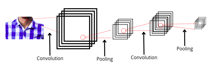
A convolutional neural network can have tens or hundreds of layers that each learns to detect different features of an image. Filters are applied to each training image at different resolutions, and the output of each convolved image is used as the input to the next layer. In the context of a convolutional neural network, convolution is a linear operation that involves the multiplication of a set of weights with the input, much like a traditional neural network.

Given that the technique was designed for two-dimensional input, the multiplication is performed between an array of input data and a two-dimensional array of weights, called a filter or a kernel. We will learn more about the filters in the upcoming sections but before it, let us learn the structure of different images.

Different types of images

The three most common types of images used in convolutional neural networks are:

• Binary image
• Grayscale image
• Colored image

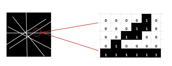
A binary image is an image that contains exactly two colors, such as white and black. Binary images are also called bi-level or two-level. Each pixel is stored as a single bit- 0 or 1 as shown below.

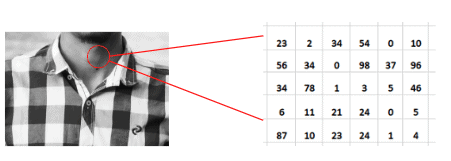
While a Grayscale image is an image that contains a range(0, 255) of shades of gray without the color, the darkest possible shade is black, and the lightest possible shade is white. The matrix of grayscale image data represents intensities within some range, as shown below:

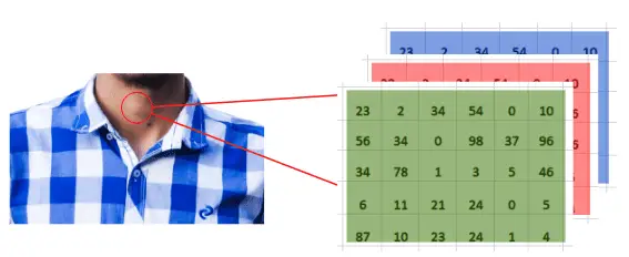
While colored images, also known as RGB, can be viewed as three different images(a red scale image, a green scale image, and a blue scale image) stacked on top of each other. Such images are more complex as they contain more information. The sample image below shows an RGB image.

Now, let us understand the key terms used in a convolutional neural network to extract information from the images.

What is padding in a convolutional neural network?

Convolution is a mathematical way of combining two signals to form a third signal. But in Artificial Neural Networks, it is fundamental to many common image processing operators. Convolution provides a way of multiplying two arrays/matrices of numbers, generally of different sizes, but producing a third array of numbers of the same dimensionality.

Let’s assume we have the following two matrices, multiplying to get the third matrix.

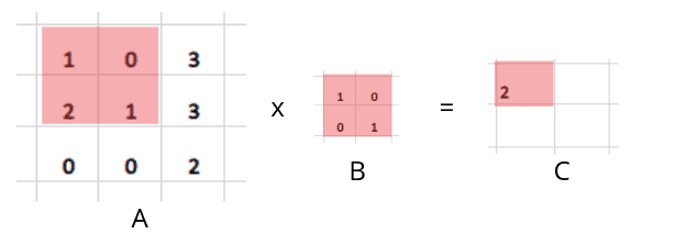
In image processing, matrix A represents information about an image, and matrix B is any filter. In image processing, filters are mainly used to suppress either the high frequencies in the image, i.e., smoothing the image, or the low frequencies, i.e., enhancing or detecting edges in the picture. But as you can see, when we applied filtering to the above image ( multiplied A with B), we got fewer dimensions than the original image. The original image was 3×3; after applying a filter to detect high or low frequencies in an image, it reduces to a 2×2 matrix. This is where the padding comes to help us.

Padding describes the addition of empty pixels around the edges of an image. The purpose of padding is to preserve the original size of an image when applying a convolutional filter and enable the filter to perform full convolutions on the edge pixels. For example, see the image processing below, where we applied filtering and padding on an image ( Matrix A) to obtain the same size result.

As you can see, our original matrix size was 3×3, but we added a new layer of empty pixels around the image (padding) and then applied it to the filter to get an image size of 3×3 again.

What is pooling in a convolutional neural network?

Pooling in convolutional neural networks is a technique for generalizing features extracted by convolutional filters and helping the network recognize features independent of their location in the image. The main purpose of the pooling layer is to progressively reduce the spatial size of the input image, reducing the number of computations in the network. Pooling downsamples by reducing the size and sending only the important data to the next layers in CNN.

There are two types of pooling in a convolutional neural network; Max Pooling and Average Pooling. In max pooling, we consider only the maximum value for the next convolutional layer, while in average pooling, we take the average of the values. See the example below of Max pooling and Average pooling.

As you can see, in Max pooling, we only take the maximum value for the next layer, while in average pooling, we take the average of the values for the next layer. Both of them reduce the size of the image while retaining important information.

The architecture of the fully connected layer of CNN

Now we have a basic understanding of how different processes are performed on the matrix of images in CNN. Let us now understand the fully connected convolutional neural network step by step.

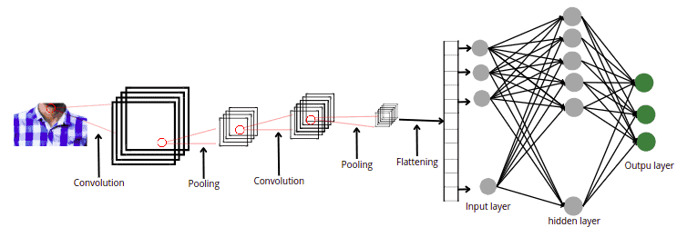
Like any other neural network, a convolutional neural network consists of an input, an output layer, and multiple hidden layers. The hidden layers of a CNN typically consist of a series of convolutional layers that convolve with multiplication or other dot product, and ReLU is mainly applied as an activation function. The ReLU activation function is used because it converts any negative value to zero. We know the image matrix cannot contain negative values, so if there are any negative values in the matrix because of processing, the ReLU function will transform them into non-negative values.

Once we are done with the filtering and pooling process, the last step before feeding the image to the neural network is to flatten the matrix. The flattening step is a refreshingly simple in building a convolutional neural network. It involves taking the pooled feature map generated in the pooling step and transforming it into a one-dimensional vector. So, in simple words, flattening converts an NxN matrix into a one-dimensional array.

The following figure shows the full architecture of CNN, from image processing to feeding to the neural network.

We will now build a convolutional neural network in TensorFlow on the grayscale and colored image using the abovementioned steps.

Tensorflow CNN – Classification of Grayscale images

Now, we will jump into the implementation part and build a convolutional neural network to help classify grayscale images. In this section, we will be using the Fashion MNIST dataset. The dataset contains 70000 examples. Each example is a 28×28 grayscale image associated with a label from 10 classes. You can read more about the dataset from this link.

Before implementing, ensure you have installed the following Python modules on your system.

• TensorFlow
• Keras
• NumPy
• matplotlib
• pandas

We recommend installing Jupyter Notebook and executing the following commands in the cell of the Jupyter Notebook:

%pip install tensorflow
%pip install numpy
%pip install keras
%pip install pandas
%pip install matplotlib

Once the installation is complete, we can move to the practical part.

Importing and exploring the dataset

The Fashion MNIST dataset is inside the submodule of TensorFlow. We can quickly load it from there.

# importing TensorFlow
import tensorflow as tf
# loading the fashion mnist data
fashion_mnist = tf.keras.datasets.fashion_mnist

We will assign the training and testing data to respective variables in the next step.

# Splitting the dataset into testing and training parts
(train_images, train_labels), (test_images, test_labels) = fashion_mnist.load_data()

Let us now check the shape of the training dataset and labels.

#shape of dataset
print(train_images.shape)
print(train_labels.shape)

Output:

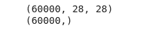
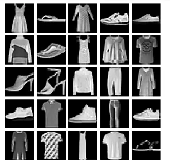
As you can see, there is a total of 60000 images, each containing a 28×28 matrix. Now, let us visualize each of the images available in the dataset.

# importing the modules
import matplotlib.pyplot as plt
import numpy as np
#ceating columns and rows 
columns = 5
rows = 5
# fixing the size of plot
fig = plt.figure(figsize=(8, 8))
# using for loop to iterate
for i in range(1, columns * rows+1):
    data_idx = np.random.randint(len(train_images))
    img = train_images[data_idx].reshape([28, 28])
    fig.add_subplot(rows, columns, i)
    plt.imshow(img, cmap='gray')
    plt.axis('off')
plt.tight_layout()
plt.show()

Output:

Now, we will apply a simple preprocessing step because if we inspect an individual image, we will see that the pixel values fall in the range of 0 to 255, as shown below:

# plotting one image frrom the data
plt.figure()
plt.imshow(train_images[1], cmap='gray')
# printing the color bar
plt.colorbar()
plt.grid(False)
plt.show()

Output:

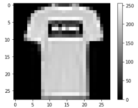
As you can see, the pixel values are from 0 to 255. We will scale these values from 0 to 1 before feeding them to the neural network model.

# divide by 255 to range from 0 to 1
train_images = train_images / 255.0
test_images = test_images / 255.0

With this, our data is ready to be used for a Convolutional neural network.

Building convolutional neural network

We will now use the TensorFlow module to build the CNN. Let us first initialize the model with one hidden layer.

# initializing the model
model = tf.keras.Sequential([
    # flattening the layers to have an image size of 28x28
    tf.keras.layers.Flatten(input_shape=(28, 28)),
    # Adding dense layer with 128 nodes
    tf.keras.layers.Dense(128, activation='relu'),
    # adding output  layer with 10 nodes
    tf.keras.layers.Dense(10)
])

The first layer Flatten, transforms the format of the images from a two-dimensional array (of 28 by 28 pixels) to a one-dimensional array. Then we added a hidden layer consisting of 128 nodes, and the activation function is ReLU. The last layer is the output layer, and as you can see, we have specified the number of nodes as 10 as we have a total of 10 categories of output data.

The next step is to compile the above-created neural network. The compiling model requires three main parameters.

The loss function measures how accurate the model is during training. The optimizer is used to update the model based on the data it sees and its loss function. And finally, the matrice is used to monitor the training and testing steps. So, now let us compile the model using these parameters.

# compiling the model
model.compile(optimizer='adam',
              loss=tf.keras.losses.SparseCategoricalCrossentropy(from_logits=True),
              metrics=['accuracy'])

Training and testing the model

Now we will train the model using the training dataset. We will fix the epoch value to be 10. You can change this value to get an optimized result.

# training the model
model.fit(train_images, train_labels, epochs=10)

Once the training is complete, we can then use the testing data to find the accuracy of the classifications.

# finding the test accuracy
test_acc = model.evaluate(test_images,  test_labels)
# printing the accuracy
print('Test accuracy:', test_acc[1])

Output:

As you can see, we got an accuracy score of 87%, which means our model could classify 87% of the testing data correctly.

Check how to apply parameter tuning to the classification problem in the An easy introduction to Artificial Neural Networks article.

Classification of colored images using TensorFlow

Now, we will create a convolutional neural network to classify colored images using TensorFlow. As we know, colored images are more complex and contain more information, so here we will learn how to add filters and pooling process in TensorFlow.

In this section, we will be using CIFAR images. The dataset consists of 60000 32×32 color images in 10 classes, with 6000 images per class. There are 50000 training images and 10000 test images. You can read more about the dataset from this link.

Loading and exploring the dataset

TensorFlow’s datasets module also contains colored images. So, we will load it from there and split it into training and testing parts.

# loading both trained and test data
(train_images, train_labels), (test_images, test_labels) = tf.keras.datasets.cifar10.load_data()

Now, let us check the shape of the training dataset.

# printing the shape 
print(train_images.shape)

Output:

This shows that our dataset contains 50000 examples of 32×32 matrix, and the 3 show that they are RBG/colored images.

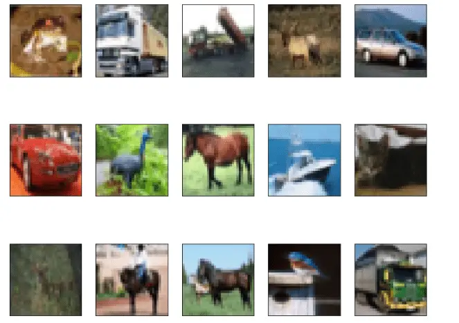
Now, let us plot the first 15 images from the training dataset.

# figure size
plt.figure(figsize=(12,10))
# looping for first 15 images
for i in range(15):
    plt.subplot(3,5,i+1)
    plt.xticks([])
    plt.yticks([])
    plt.grid(False)
    plt.imshow(train_images[i])
plt.show()

Output:

We will also scale the images to have values from 0 to 1 by dividing 255.

# Normalize 0 and 1
train_images, test_images = train_images / 255.0, test_images / 255.0

Now, let us understand how pooling and padding are useful and how they affect the size of images.

Understanding the effect of padding and pooling

Before building the convolutional neural network, we will apply some preprocessing techniques, including filtering and pooling, as we discussed earlier.

We will initialize the model and then apply a filter of a 3×3 matrix. We also need to specify the input image size( 32, 32, 3).

# initializing the model
model = tf.keras.models.Sequential()
# applying filter of size 3 by 3 and total of 32 filters
model.add(tf.keras.layers.Conv2D(32, (3, 3), activation='relu', input_shape=(32, 32, 3)))

We will only use the Max pooling method to get the important feature. And the size of the max-pooling matrix is 2 by 2.

# adding pooling method
model.add(tf.keras.layers.MaxPooling2D((2, 2)))

Let us summarize the model to see how the pooling and filtering have affected the images.

# model summary
model.summary()

Output:

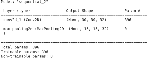
Here are two things to note. First, notice that the output shape of the matrices after filtering is 30 by 30, whereas the original size was 32 by 32. It is because we didn’t apply any padding method. Secondly, as you can see, the pooling has even reduced the size to 15 by 15.

Let us now create another model, apply the same steps above with padding and see the differences.

# initializing the model
model1 = tf.keras.models.Sequential()
# applying filter of size 3 by 3 and total of 32 filters
model1.add(tf.keras.layers.Conv2D(32, (3, 3), padding='same', activation='relu', input_shape=(32, 32, 3)))
# adding pooling method
model1.add(tf.keras.layers.MaxPooling2D((2, 2)))
model1.summary()

Output:

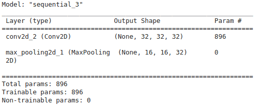
As you can see, the filtering does not affect the matrix size this time as we have applied the padding.

Building a fully connected convolutional neural network

Let us now create a fully connected convolutional neural network. We will apply filtering and max-pooling before the hidden layers.

# building model
model = tf.keras.models.Sequential()
model.add(tf.keras.layers.Conv2D(32, (3, 3), activation='relu', input_shape=(32, 32, 3)))
model.add(tf.keras.layers.MaxPooling2D((2, 2)))
model.add(tf.keras.layers.Conv2D(64, (3, 3), activation='relu'))
# flattening the input matrix
model.add(tf.keras.layers.Flatten())
# applying hidden layer with 32 nodes
model.add(tf.keras.layers.Dense(32, activation='relu'))
# output layer with 10 nodes
model.add(tf.keras. layers.Dense(10))

As you can see, we applied two filters with one pooling layer. Then we used the flattening layer to convert the input matrices to a one-dimensional array. We also have assigned 32 nodes in the hidden layer and 10 nodes in the output layer, as there are 10 different categories in the output class.

Now, we will compile and train the model on the training images.

# compiling the model
model.compile(optimizer='adam',
              loss=tf.keras.losses.SparseCategoricalCrossentropy(from_logits=True),
              metrics=['accuracy'])
# fitting model
model.fit(train_images, train_labels, epochs=10)

As you can see, we have specified the epochs to be 10. You can change this value to get the optimum result or use the parameter tuning method to get the optimum epoch value.

Let us also test our model and find out the accuracy score.

# finding the test accuracy
test_acc = model.evaluate(test_images,  test_labels)
# printing the accuracy
print('Test accuracy:', test_acc[1])

Output:

As you can see, we get an accuracy score of 67%, which is pretty low. The reason is that we have randomly selected the number of the hidden layer, nodes, and epoch value. You can use the tunning parameter method to find the optimum values for these parameters and get a better result.

Summary

Convolutional Neural Network or CNN is a type of artificial neural network widely used for image/object recognition and classification. In this article, we learned how to build a convolutional neural network and how it works. We also used TensorFlow to make a predictive model for grayscale and colored images.