LightGBM algorithm: Supervised Machine Learning in Python

LightGBM is a Supervised ensemble Machine Learning algorithm. It works in a similar way as XGBoost or Gradient Boosting algorithm does but with some advanced and unique features. In this article, we will discuss how the LightGBM boosting algorithm works and how it differs from other boosting algorithms. We will also apply the LightGBM algorithm using Python to solve classification and regression problems. We will use AWS SageMaker Studio and Jupyter notebooks for implementation and visualization purposes.

We assume that you already have a solid understanding of Random Forests and Decision Tree models as the LightGBM uses Random Decision trees for boosting. Also make sure that you have some knowledge about the Gradient boosting, CatBoost, and XGBoost algorithms as well because they work in a similar way and we will also compare them with LightGBM in this article.

Key features of the LightGBM algorithm

Here are some of the key features of LightGBM that make it one of the unique boosting algorithms:

• It takes care of the missing values automatically – that means we don’t need to do any preprocessing steps to handle missing values.
• It uses a histogram-based algorithm for splitting to create split points – split points are the feature values depending on which data is divided at a decision tree node.
• It uses Gradient-Based One Side Sampling (GOSS) which is a novel sampling way that downsamples the instances on basis of gradients.
• The decision trees in LightGBM are leaf-wise tree growth. The difference between leaf-wise tree growth and level-wise tree growth is that the leaf-wise strategy grows the tree by splitting the data at the nodes with the highest loss change, and the level-wise strategy grows the tree level by level.
• Another feature of LightGBM is that it uses the Exclusive Feature Bundle Technique, which is a near-lossless method to reduce the number of effective features.
• Faster training speed and higher efficiency. Lower memory usage and better accuracy.

NOTE: Some of the terms may not be clear right now, don’t worry we will explain them in the next section in more detail.

Explanation of LightGBM algorithm

LightGBM (Light Gradient Boosting Machine) is an open-source library that provides an efficient and effective implementation of the gradient-boosting algorithm. It was developed by Microsoft company and was made publically available in 2016. It works in a similar way as other boosting algorithms but with some advanced features which makes it one of the fasted boosting algorithms.

The very first feature that has a key role in making LightGBM fast is histogram-based splitting. Let us take sample data to understand how the histogram-based splitting makes the algorithm faster. We assume that we have a dataset of salaries of a few employees.

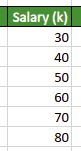
To create an optimal spit for a Decision tree, all the above values in the dataset will be tested. Suppose we have millions of data rows, then it takes a lot of time to test for the best split. The LightGBM solves this issue in an optimal way. It divides the dataset into different bins. For example, let’s say in our case, it divides the above dataset into two bins.

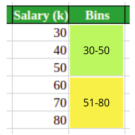
Now, instead of testing all the data points for the optimum splitting, the LighGBM will use the bins to find the optimum split which takes less time.

The second feature that has a great role in making the LightGBM faster is the Exclusive Feature Bundling (EFB) Technique. It helps to decrease features that are sparse. Exclusive Feature bundling (EFB) puts two features together and adds offset to every feature in feature bundles. For example, take the following categorical dataset about gender.

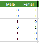
Notice that we have two columns that show the gender of a person. Instead of using both the columns, the EFB will use one column that will contain the same information as shown below:

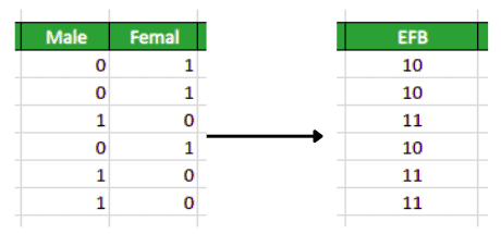
Note that the value for males is 10 and for females is 11. This is how the EFA reduces the features so that the model can easily be trained on the dataset.

The third main feature that brings more power to the LightGBM is the GOSS (Gradient-Based One Side Sampling). The gradient is simply a derivative or the function’s rate of change. The large value of the gradient shows more error. LightGBM uses the technique of Gradient-based One-Side Sampling to reduce the number of training examples. The GOSS keeps all the examples with large gradients (error) and conducts random sampling on the examples with small gradients. In other words, the models keep the observations/data points for the next iteration that has a high gradient value so that it can reduce the error.

The above-mentioned features helped the LightGBM algorithm to build a random forest of Decision trees in less time to make predictions and to improve the error rate.

LightGBM Ensemble for Regression using Python

Let’s apply the LightGBM regressor to solve a regression problem. A dataset having continuous output values is known as a regression dataset. In this section, we will use the dataset about house prices. The input variables are the number of rooms, the number of floors, the area, and the location of the houses, and the target variable is the price of houses. You can get access to the dataset from this link.

Before going to the implementation part, make sure that you have installed the following Python modules as we will be using them in the implementation.

• lightGBM
• sklearn
• pandas
• numpy
• matplotlib

You can install them on your system by running the following commands in the cell of the Jupyter notebook.

%pip install lightgbm
%pip install sklearn
%pip install pandas
%pip install numpy
%pip install matplotlib

Once the installation is complete, we can then move to the implementation part.

Importing and exploring the dataset

Let us now use the Pandas DataFrame class to import the dataset and print a few rows to get familiar with the type of the dataset:

# importing the module
import pandas as pd
# importing tabular data
dataset = pd.read_csv('Dushanbe_house.csv')
# printing few rows
dataset.head()

Output:

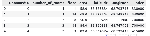
As you can see the dataset has some NULL values, we will not handle them in the preprocessing part as the LightGBM can handle them automatically.

We will drop the column Unnamed: 0, as it contains the index values which do not have any relation with the output values.

# dropping the column
dataset.drop('Unnamed: 0', axis=1, inplace=True)

Now, we can use the Pandas DataFrame info() function to get more information about the dataset.

# pandas info
dataset.info()

Output:

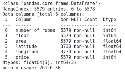
Note that we have a total of 5579 observations and the number of features is 6.

Let’s plot the boxplots for each of the features to see the distribution of the data points.

# importing the modules
from plotly.subplots import make_subplots
import plotly.graph_objects as go
# fixing the subplots
fig = make_subplots(rows=2, cols=2)

# box plot for price
fig.add_trace(go.Box(y=dataset.price.values,name="Price"),row=1, col=1)
# box plot of area
fig.add_trace(go.Box(y=dataset.area.values,name="Area"),row=1, col=2)
# box plot of floors
fig.add_trace(go.Box(y=dataset.floor.values,name="Floor"), row=2, col=1)
# box plot of rooms
fig.add_trace( go.Box(y=dataset.number_of_rooms.values,name="Number of rooms"), row=2, col=2)
# plotting
fig.update_layout(height=700, width=1000, title_text="Boxplot of the data")
fig.show()

Output:

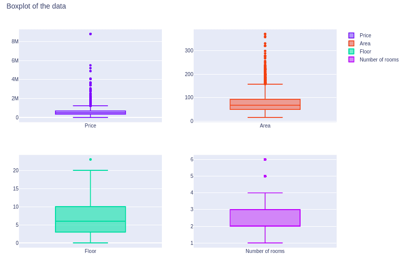
The above chart shows that there are some outliers in each of the features. If you want to know how to detect the outliers and handle them, please go through the Implementation of Isolation Forest and Anomaly detection using Python articles.

Splitting the dataset

We need to divide the dataset into input features and output variables. Note that in our case, the price column is going to be our target variable as we will be building a model using LightGBM to predict the price of the house.

# taking the columns from the dataset
columns = dataset.columns
# storing the input and output variables
Inputs = dataset[columns[0:-1]]
outputs = dataset[columns[-1]]

Now we can split the dataset into training and testing parts so that we can train the model and then evaluate the performance of the model using the testing dataset. We will use the sklearn module for splitting the dataset.

#Train and testing data
from sklearn.model_selection import train_test_split
# assign test data size 25%
X_train, X_test, y_train, y_test =train_test_split(Inputs,outputs,test_size= 0.25, random_state=0)

We have assigned 75% of the data for the training and the remaining 25% for the testing part.

Training and evaluation of LightGBM regressor

We will now import the LightGBM regressor and train the model using the training data set. We will use all the default values for the parameters.

# import lightgbm
import lightgbm as lgb
# initialzing the model
model = lgb.LGBMRegressor()
# train the model
model.fit(X_train,y_train)

Once the training is complete, we can use the testing data to predict the target variable.

# Making predictions
lightR_predict = model.predict(X_test)

Now it is time to use different ways to evaluate the performance of the model.

We will first visualize both the predictions and the actual values to see how they are close to each other. We will use the Matplotlib module for the visualization of the predictions.

# importing the module
import matplotlib.pyplot as plt
# fitting the size of the plot
plt.figure(figsize=(15, 8))
# plotting the graphs
plt.plot([i for i in range(len(y_test))],y_test, label="actual values")
plt.plot([i for i in range(len(y_test))],lightR_predict, label="Predicted values")
# showing the plotting
plt.legend()
plt.show()

Output:

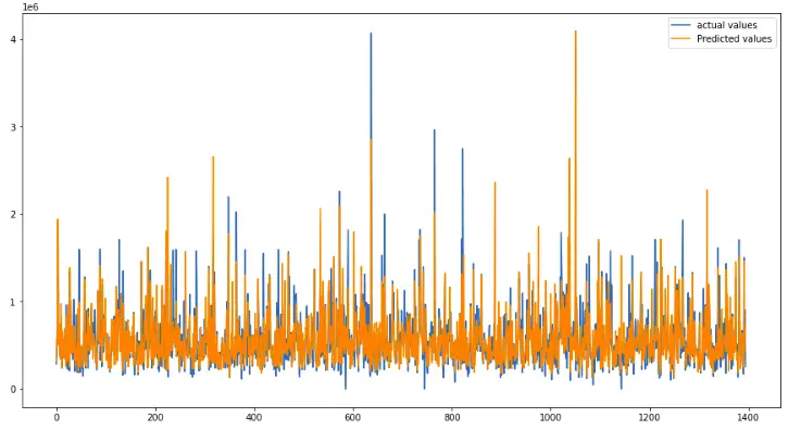
The plot shows that the predictions and the actual values are close enough and the model was successful to follow the trend in the dataset.

Let’s visualize the data again by plotting the mean of the training data and testing data to see how much they differ from each other.

# fitting the size of the plot
plt.figure(figsize=(15, 8))
# printing the mean 
print("Mean of actual values : ", y_test.mean())
print("Mean of predicted values: ", lightR_predict.mean())
# plotting the graphs
plt.plot([i for i in range(len(y_test))],y_test, label="actual values")
plt.plot([i for i in range(len(y_test))],lightR_predict, label="Predicted values")
plt.plot([i for i in range(len(y_test))],[y_test.mean() for x in range(len(y_test))], label = "mean of actual values")
plt.plot([i for i in range(len(y_test))],[lightR_predict.mean() for y in range(len(y_test))], label = 'mean of predicted values')
# showing the plotting
plt.legend()
plt.show()

Output:

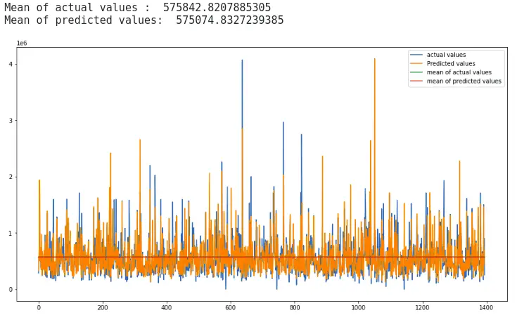
As you can see, the mean of the actual values and the predictions are very close which shows the model was making predictions close to the actual values.

Now let’s also find the R²-score of the model. R²-score shows how close the predictions are to the actual values. The value of the R²-score is usually between 0 and 1. The closer the value is to the 1, the better the predictions are.

# Importing the required module
from sklearn.metrics import  r2_score
# Evaluating model performance
print('R-square score is :', r2_score(y_test, lightR_predict))

Output:

Note that the R²-score value shows our predictions were pretty close to the actual values. You can even apply GridSearchCV to improve the efficiency of the model.

Comparing LightGBM with other boosting algorithms

As you have seen, by using the default parameter values, we get very good results. Now we will compare the performance of the LightGBM model with other boosting models. We will use the same dataset (the price of houses), to train the boosting model and then compare their R²-score values.

LightGBM vs XGBoost Machine learning algorithm

As we have already implemented LightGBM on the above-given dataset and calculated the R²-score value. Now we will use the XGBoost (extreme gradient boosting) algorithm to train the model and will compare the results. If you want to know how the XGBoot algorithm works and how it differs from the LightGBM, please go through the Implementation of XGBoost using Python.

Let’s train the model and make predictions using the testing dataset.

# importing the module
import xgboost as xgb
# we initiate the regression model and train it with our train data
xg_reg = xgb.XGBRegressor()
# train the model
xg_reg.fit(X_train,y_train)
# making prediction
xg_prediction = xg_reg.predict(X_test)

Once the training is complete, we can calculate the R²-score of the XGBoost with the R²-score score of the LightGBM.

# Evaluating model performance
print('R-square score of LightGBM is :', r2_score(y_test, lightR_predict))
print('R-square score of XGBoost  is :', r2_score(y_test, xg_prediction))

Output:

Note that the value of the R²-score for the XGBoost is less than that of LightGBM, which shows on the given dataset, that LighGBM performed well as compared to the XGBoost.

LightGBM vs CatBoost Machine Learning algorithm

Now let’s compare the LightGBM with the CatBoost algorithm, one of the recent resembling algorithms. You can read how it makes predictions and differs from LightGBM in the CatBoost: Supervised machine learning algorithm article.

Let’s import the model and train on the training dataset.

# importing the required module
from catboost import CatBoostRegressor
# initializing the model
cbr = CatBoostRegressor()
# train the model
cbr.fit(X_train, y_train)
# prediction
cbr_prediction = cbr.predict(X_test)

Once the training and predictions are complete, we can then calculate the R²-score score and compare it with LightGBM.

# Evaluating model performance
print('R-square score of LightGBM is :', r2_score(y_test, lightR_predict))
print('R-square score of CatBoost  is :', r2_score(y_test, cbr_prediction))

Output:

This shows that both the algorithms performed well but again the predictions of LightGBM were better CatBoost model on our dataset.

LightGBM vs Gradient Boosting decision tree algorithm

Now we can train the model using the Gradient boosting algorithm and compare the results. One of the limitations of Gradient Boosting is that it cannot handle the null values and our dataset contain null values. So, if we use the dataset without any preprocessing step to handle the Null values, the training part will give errors. For that reason, we will be using the preprocessed (dropped null values) version of the dataset. If you want to know how the gradient boosting algorithm works and how to preprocess the dataset to handle Null values, please read the Implementation of the Gradient Boosting algorithm using Python article.

Let’s train the model on the preprocessed data and make predictions using the testing dataset.

# Importing the Gradient Boosting Regressor machine learning algorithm
from sklearn.ensemble import GradientBoostingRegressor
# train machine learning algorithms
GB_regressor=GradientBoostingRegressor()
#gradient boosting framework train
GB_regressor.fit(X_train,y_train)
# prediction
GB_predict=GB_regressor.predict(X_test)

Once the training and predictions are complete, we can calculate the R²-score score and compare it with the LightGB.

# Evaluating the model performance
print('R-square score of LightGBM is :', r2_score(y_test, lightR_predict))
print('R-square score of Gradient boosting is :', r2_score(Y_test, GB_predict))

Output:

Note that the R²-score score of LightGBM is again higher than the R²-score score of the Gradient boosting algorithm, which means on the given dataset, LightGBM performed well than the Gradient Boosting algorithm.

LightGBM Ensemble for Classification using Python

Now we can apply the LightGBM classifier to solve a classification problem. The dataset is about the chess game. You can get access to the dataset from this link.

The kr-vs-kp.names file contains all the necessary information about the dataset. It is highly recommended to read the information in this file to get yourself familiar with the dataset. The output class has two possible outcomes: White-can-win (“won”) and White-cannot-win (“nowin”).

Before applying the LightGBM classifier to the dataset, let’s import the dataset and explore it.

Importing and exploring a dataset

We will import the dataset using the Pandas module and will print a few rows to get familiar with the type of data points.

# importing the dataset
data = pd.read_csv('kr-vs-kp.data')
# printing few columns
data.head()

Output:

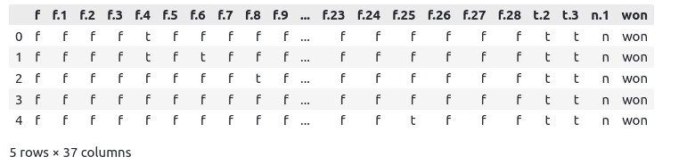
The last column contains the target class while the rest of the 36 columns describe the chessboard (Go through kr-vs-kp.names to read more about the type of data).

As you can see, the heading is also missing. Let us add the headings that are described in the kr-vs-kp.names file.

# many features 
attributes = ['bkblk','bknwy','bkon8','bkona','bkspr','bkxbq','bkxcr','bkxwp','blxwp','bxqsq','cntxt','dsopp','dwipd','hdchk','katri','mulch','qxmsq','r2ar8','reskd','reskr','rimmx','rkxwp','rxmsq','simpl','skach','skewr',
 'skrxp','spcop','stlmt','thrsk','wkcti','wkna8','wknck','wkovl','wkpos','wtoeg', 'Target']
# adding heading to the dataframe / feature values
data.columns = attributes
# dataset
data.head()

Output:

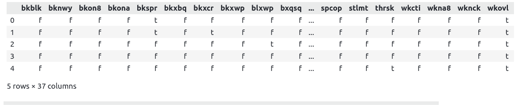
As you can see that the dataset contains object values (non-numeric). We will not apply LabelEncoding/one hot encoding methods to convert the non-numeric values to numeric. We just need to convert these object datatype to categorical values because LightGBM automatically converts the categorical values to numeric values.

# converting datapoints to categorical features
for feature in attributes:
    # categorical features
    data[feature] = pd.Series(data[feature], dtype="category")

Splitting the dataset

We will now divide the dataset into input and output variables.

# taking the columns from the dataset
columns = data.columns
# storing the input and output variables
Inputs = data[columns[0:-1]]
outputs = data[columns[-1]]

Now we can split the dataset into the training and testing parts.

# assign test data size 30%
X_train, X_test, y_train, y_test =train_test_split(Inputs,outputs,test_size= 0.3, random_state=0)

We have assigned70% of the data for the training part. Let us now check the sizes of the testing and training parts.

print("shape of training data : ", X_train.shape)
print("shape of testing data : ", X_test.shape)

Output:

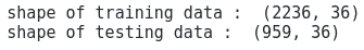
This shows our training data contain 36 features. Also, we will use 2236 train the model and 959 observations to test the model

Training and evaluating the performance of the LightGBM Classifier

Let us now import the classifier and train it on our dataset.

# this parameter converts the categorical values to numeric values (not one hot encoded features)
fit_params={'categorical_feature': 'auto'}
# lightgbm import lgbmclassifier machine learning algorithm
lightClf = lgb.LGBMClassifier()
# train the final model and important parameters
lightClf.fit(X_train, y_train, **fit_params)

Note that training the model takes one extra parameter as well which specifies converting the categorical values to numeric values before training the model.

We will now use the testing data to make predictions.

# making prediction 
light_prediction = lightClf.predict(X_test)

Once the predictions are done, we will use the confusion matrix to evaluate the performance of the model.

# importing seaborn
import seaborn as sns
# Making the ConfusionMatrix
from sklearn.metrics import confusion_matrix
# setting the size
sns.set(rc={'figure.figsize':(10,8)})
# providing important parameters
cm = confusion_matrix(y_test, light_prediction)
sns.heatmap(cm,annot=True)
# saving confusion matrix in png form
plt.savefig('confusion_Matrix.png')

Output:

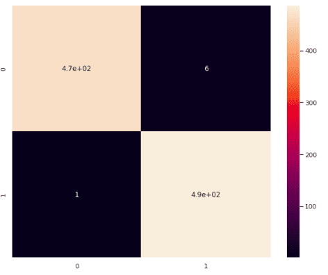
This shows that out of 959 only 7 values are misclassified by the model. The rest all have been classified correctly,

Let’s also calculate the accuracy scores as well.

# importing accuracy score
from sklearn.metrics import accuracy_score
# printing the higher accuracy /better performance rate
accuracy_score(y_test, light_prediction)

Output:

This shows that 99% of the testing data has been correctly classified by the LightGBM model on the given classification data.

Summary

In this article, we have discussed the LightGBM algorithm in detail. We have seen how it works and differs from other boosting algorithms like XGBoost or Gradient Boosting. We also applied the LightGBM algorithm to a few classification and regression problems to see how well it performed. The impressive results showed that a LightGBM algorithm is a powerful tool for solving Machine Learning problems.