CatBoost algorithm: Supervised Machine Learning in Python

The CatBoost algorithm is a Supervised Machine Learning algorithm developed by Yandex researchers and engineers. It is used for search, recommendation systems, personal assistants, self-driving cars, weather prediction, and many other tasks. This article will review the CatBoost algorithm’s powerful features and apply it to the demo datasets to solve classification and regression problems.

Before starting the article, ensure you have a solid understanding of the Gradient Boosting and XGBoost algorithms. We also assume that you understand the Decision Trees and Random Forests algorithms.

Best Machine Learning Books for Beginners and Experts

As Machine Learning becomes more and more widespread, both beginners and experts need to stay up to date on the latest advancements. For beginners, check out the best Machine Learning books that can help to get a solid understanding of the basics. For experts, reading these books can help to keep pace with the ever-changing landscape. In either case, a few key reasons for checking out these books can be beneficial.

First, they provide a comprehensive overview of the subject matter, mainly about Machine Learning algorithms. Second, they offer insights from leading experts in the field. And third, they offer concrete advice on how to apply Machine Learning concepts in real-world scenarios. As Machine Learning continues to evolve, there’s no doubt that these books will continue to be essential resources for anyone with prior knowledge looking to stay ahead of the curve.

Key features of the CatBoost algorithm

Here are some of the key features of the algorithm:

• The algorithm automatically takes care of NULL values in the dataset
• The algorithm automatically does label encoding for categorical features
• The algorithm uses binary symmetric decision trees

Explanation of CatBoot algorithm

The CatBoost (Categorical Boosting) algorithm is one of the newest boosting algorithms (published in 2017). This algorithm is designed to work with categorical features, and it works similarly to Gradient and XGboost algorithms. Still, it has some advanced features which make it more reliable, fast, and accurate. Let’s illustrate how the algorithm works using a sample dataset.

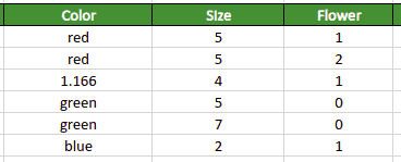
Our sample dataset contains data about three different flowers represented by their size and color:

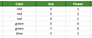
Most Machine Learning algorithms require only numerical features for the training process, so If you try to use this dataset “as is” without prior preprocessing, you’ll not be able to do it. You must convert categorical features’ values (the “Color” column in our example) into numeric values. Such conversion is called label encoding.

Label encoding is one of the data pre-processing steps in Machine Learning workflow responsible for converting categorical feature variables (labels) into numerical values. For example, if the feature variable “color” (column) in the dataset represented by the “red”, “green” and “blue” colors, the label encoding process will replace all red color values in the dataset with numeric value 1, green color values with the numeric value 2, and blue color values with the numeric value 3.

The scikit-learn Python contains the LabelEncoder helper class that handles this process for you automatically.

The robust feature of the CatBoost is that it automatically handles categorical features in a very optimized way.

For example, suppose, as part of the preprocessing process, we want to apply traditional label encoding to the “color” feature (column). In that case, we’ll get the following expected result:

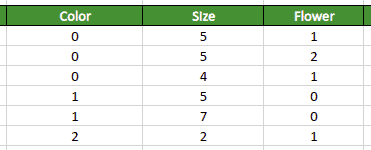
When it comes to the CatBoost algorithm, it automatically handles label encoding in its own creative and optimized way. The algorithm converts categorical features by finding the feature relationship with the output class. The CatBoost algorithm does label encoding using the following formula:

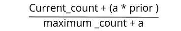
In the above equation:

• a and prior are the constant parameters, by default, equal to 1 and 0.5
• Current_count is the sum of all the output class values of the same category that the current row in the dataset belongs to
• maximum_count is the sum of the same category items above the current row

Let’s illustrate how to calculate the equation above. Let’s assume we are converting the third-row item (highlighted using light-blue color):

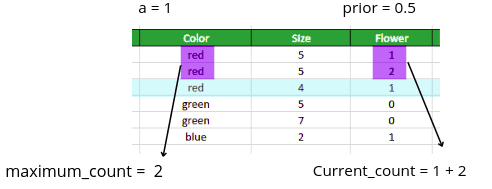
As soon as we have values of all required variables, we can convert the categorical feature in the third row:

Numeric Value = (1 + 2) + ( 1 * 0.5 ) / ( 2 + 1)

Numeric value = 1.166

The algorithm applies its version of the label encoding process to all categorical data and handles categorical variables of the entire dataset using the same formula.

In the case of traditional label encoding, all rows containing the “red” value in the “Color” column will have the same numeric value. In the CatBoost algorithm’s case, the “red” value in the “Color” column will not necessarily have the same value for every row in the dataset.

Similar to the Gradient Boosting and XGBoost algorithms, the CatBoost algorithm creates several Binary Decision Trees each time trying to reduce the error:

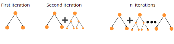
Once all iterations are complete, the algorithm stops creating new decision trees and finds the best-fitted model using the already familiar approach.

Solving a regression problem

Let’s apply CatBoost’s regressor to the regression dataset. The dataset contains the price information of houses in Dushanbe city. The input variables are the number of rooms, floors, area, and location. You can download the dataset using the following link.

Before going to the implementation part, ensure that you have installed the required Python modules.

• catboost
• pandas
• numpy
• matplotlib

You can install the required modules by running the following commands in the cell of the Jupyter notebook,

%pip install catboost
%pip install pandas
%pip install numpy
%pip install matplotlib

The Pandas, NumPy, and Matplotlib modules should already be familiar to you. The only difference this time is in the CatBoost library (link). The CatBoost library can be used to solve both classification and regression problems. For classification, you can use CatBoostClassifier. For regression will require CatBoostRegressor.

Once the modules are installed, we can go to the implementation part.

Importing and exploring the dataset

We will use the Pandas DataFrame to store the imported dataset. Let’s import the Pandas module and then use read_csv() method to load the data.

# importing the module
import pandas as pd
# importing dataset
dataset = pd.read_csv("Dushanbe_house.csv")

Let’s print a few rows of the dataset to get familiar with it:

# heading 
dataset.head()

Output:

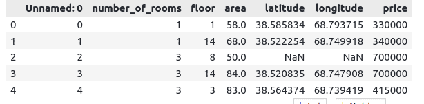
Our dataset contains one unnecessary column called ‘Unnamed: 0’ (rows indexes). In addition to that, some data items contain NULL values (imported as NaN).

Let’s remove the unnecessary index column but will keep items with NULL values in the dataset, as the algorithm will handle them automatically.

# dropping the column
dataset.drop('Unnamed: 0', axis=1, inplace=True)

Now we can use the correlation matrix to see the correlation between the variables. A correlation matrix is a table that displays the correlation (the numerical representation of dependencies of variables from each other).

If two variables are highly correlated, we can remove one as they will have the same effect on the output class. In the ideal case, you need to use only those input variables that demonstrate a linear relationship with each other.

The Pandas DataFrame’s corr() method displays the correlation table for all variables of the dataset.

# finding the correlation
dataset.corr()

Output:

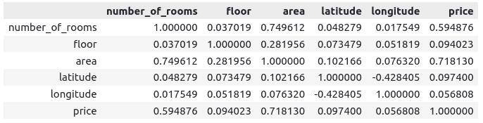
Notice that all variables have positive correlations except longitude and latitude.

Let’s visualize the variables’ correlation using the Matplotib and Seaborn libraries:

# importing required module 
import seaborn as sns
import matplotlib.pyplot as plt
# finding the correlation
corrMatrix = dataset.corr()
# size of the plot
plt.figure(figsize=(12, 6))
# correaltion matrix
sns.heatmap(corrMatrix, annot=True)
plt.show()

Output:

Notice that only latitude and longitude have a negative correlation. Moreover, there are no highly correlated variables in the dataset, so we will keep our dataset as-is.

Splitting the dataset

One of the essential parts of building Machine Learning models is splitting the dataset into testing and training parts so we can train and then evaluate the model. Let’s split the dataset into the input features and output class variables first:

# split the data into inputs and outputs
# taking the columns from the dataset
columns = dataset.columns
# storing the input and output variables
X = dataset[columns[0:-1]]
y = dataset[columns[-1]]

The next step is to split the dataset data into testing and training parts. We will use 75% of the data for training the model and the remaining 25% for testing.

#Training and testing data
from sklearn.model_selection import train_test_split
# assign test data size 25%
X_train, X_test, y_train, y_test =train_test_split(X,y,test_size= 0.25, random_state=0)

Let’s check the sizes of the testing and training datasets.

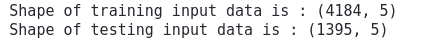
# print("Size of testing dataset'X_test.shape
print("Shape of training input data is :",X_train.shape)
print("Shape of testing input data is :",X_test.shape)

Output:

Training and testing the model

Let’s train the model. First, we must import the CatBoost regressor and then train it on the training data.

# importing the required module
from catboost import CatBoostRegressor
# initializing the model
cbr = CatBoostRegressor()
# training the model
cbr.fit(X_train, y_train)

Note that we’ve trained the model using default parameters. You check all available CatBoost algorithm parameters in the official documentation.

Once the training is complete, we can use the testing data to predict the output values:

# predictions
cbr_prediction = cbr.predict(X_test)

Let’s plot predictions and the testing data together using the Matplotlib module. You can learn how to visualize datasets using different plots from the Introduction to Matplotlib article.

# fitting the size of the plot
plt.figure(figsize=(20, 8))
# plotting the graphs
plt.plot([i for i in range(len(y_test))],y_test, label="actual values")
plt.plot([i for i in range(len(y_test))],cbr_prediction, label="Predicted values")
# showing the plotting
plt.legend()
plt.show()

Output:

The above visualization shows that the predictions are somewhat close to the actual values. Let’s find the mean of the actual and predicted values to see how exactly they are close to each other.

# fitting the size of the plot
plt.figure(figsize=(20, 8))
# printing the mean 
print("Mean of actual values : ", y_test.mean())
print("Mean of predicted values: ", cbr_prediction.mean())
# plotting the graphs
plt.plot([i for i in range(len(y_test))],y_test, label="actual values")
plt.plot([i for i in range(len(y_test))],cbr_prediction, label="Predicted values")
plt.plot([i for i in range(len(y_test))],[y_test.mean() for x in range(len(y_test))], label = "mean of actual values")
plt.plot([i for i in range(len(y_test))],[cbr_prediction.mean() for y in range(len(y_test))], label = 'mean of predicted values')
# showing the plotting
plt.legend()
plt.show()

Output:

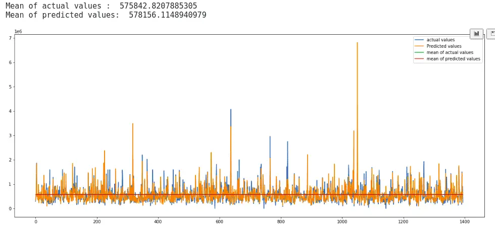
Notice that the mean of both the predictions and the actual values are very close, which shows our predictions were good enough.

We can also calculate the R²-score. The R²-score is a statistical measure representing the proportion of the variance for a dependent variable explained by an independent variable. The normal value for the R²-score is between 0 and 1. The closer the values to the 1, the better the predictions are. If the value is negative, the model failed with predictions.

# Importing the required module
from sklearn.metrics import  r2_score
# Evaluating the model
print('R-square score is :', r2_score(y_test, cbr_prediction))

Output:

The R²-score shows that predictions are good and close enough to the actual values.

Solving the classification problem

Let’s apply the CatBoost classifier to another dataset to solve the classification problem. We can use the wine dataset from the sklearn module. The dataset contains 13 different features (color, chemicals, acidity, etc.), and the output class contains two types of wines. Let’s explore the dataset to get familiar with the data.

Importing and exploring the dataset

Let’s import the dataset from the datasets a submodule of the sklearn and will print a few rows.

# importing the module
from sklearn import datasets
# loading the dataset
wine = datasets.load_wine()
# convertig the dataset into pandas dataframe
wine = pd.DataFrame(wine.data, columns=wine.feature_names)
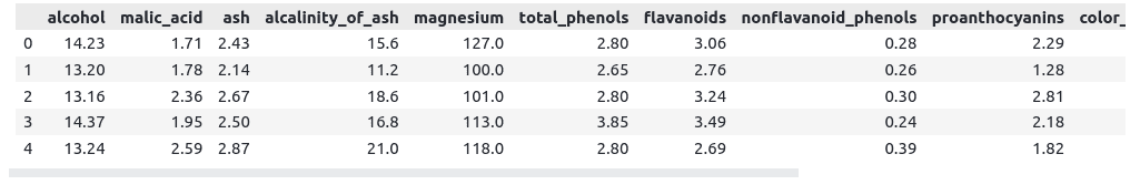
# printing rows
wine.head()

Output:

Apart from the input features, we can use the dataset’s keys to get more information about it:

# Finding the keys of the dataset
wine = datasets.load_wine()
wine.keys()

Output:

One of the import keys is DESCR, which contains the information about the dataset. It is very important to completely understand the dataset before applying any Machine Learning algorithm. Let’s print the information about the dataset:

# printing information
print(wine['DESCR'])

Output;

Wine recognition dataset
------------------------
**Data Set Characteristics:**
    :Number of Instances: 178 (50 in each of three classes)
    :Number of Attributes: 13 numeric, predictive attributes and the class
    :Attribute Information:
 		- Alcohol
 		- Malic acid
 		- Ash
		- Alcalinity of ash  
 		- Magnesium
		- Total phenols
 		- Flavanoids
 		- Nonflavanoid phenols
 		- Proanthocyanins
		- Color intensity
 		- Hue
 		- OD280/OD315 of diluted wines
 		- Proline
    - class:
            - class_0
            - class_1
            - class_2
		
    :Summary Statistics:
    
    ============================= ==== ===== ======= =====
                                   Min   Max   Mean     SD
    ============================= ==== ===== ======= =====
    Alcohol:                      11.0  14.8    13.0   0.8
    Malic Acid:                   0.74  5.80    2.34  1.12
    Ash:                          1.36  3.23    2.36  0.27
    Alcalinity of Ash:            10.6  30.0    19.5   3.3
    Magnesium:                    70.0 162.0    99.7  14.3
    Total Phenols:                0.98  3.88    2.29  0.63
    Flavanoids:                   0.34  5.08    2.03  1.00
    Nonflavanoid Phenols:         0.13  0.66    0.36  0.12
    Proanthocyanins:              0.41  3.58    1.59  0.57
    Colour Intensity:              1.3  13.0     5.1   2.3
    Hue:                          0.48  1.71    0.96  0.23
    OD280/OD315 of diluted wines: 1.27  4.00    2.61  0.71
    Proline:                       278  1680     746   315
    ============================= ==== ===== ======= =====
    :Missing Attribute Values: None
    :Class Distribution: class_0 (59), class_1 (71), class_2 (48)
    :Creator: R.A. Fisher
    :Donor: Michael Marshall (MARSHALL%PLU@io.arc.nasa.gov)
    :Date: July, 1988
This is a copy of UCI ML Wine recognition datasets.
https://archive.ics.uci.edu/ml/machine-learning-databases/wine/wine.data
The data is the results of a chemical analysis of wines grown in the same
region in Italy by three different cultivators. There are thirteen different
measurements taken for different constituents found in the three types of
wine.
Original Owners: 
Forina, M. et al, PARVUS - 
An Extendible Package for Data Exploration, Classification and Correlation. 
Institute of Pharmaceutical and Food Analysis and Technologies,
Via Brigata Salerno, 16147 Genoa, Italy.

Now we can visualize the output class to check if the data is balanced:

# defining variables
unique_values =[]
wine1=0
wine2=0
wine3=0
# for loop to iterate
for i in wine.target:
    if i ==0:
        wine1+=1
    elif i == 1:
        wine2+=1
    else:
        wine3+=1
# appending the values in a set 
unique_values.append(wine1)
unique_values.append(wine2)
unique_values.append(wine3)
# creating the names
names = ['wine 1', 'wine 2', 'wine 3']
# fixing the size of plot
plt.figure(figsize=(12, 8))
# plotting pie plot
plt.pie(unique_values, labels= names)
plt.show()

Output:

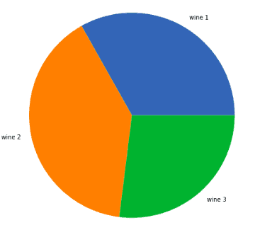
Notice that the dataset is balanced.

Training and testing the model

Before starting training the model, we need to divide the dataset into testing and training parts to train the model and then evaluate it using the testing dataset.

# splitting the data into inputs and outputs
Input, output = datasets.load_wine(return_X_y=True)
#Training and testing data
from sklearn.model_selection import train_test_split
# assign test data size 25%
X_train, X_test, y_train, y_test =train_test_split(Input,output,test_size= 0.25, random_state=0)

Let’s start model training. For simplicity, we will use the default parameters to train the classifier:

# importing the classifier
from catboost import CatBoostClassifier
# initializing the model
cbc = CatBoostClassifier()
# training the model
cbc.fit(X_train, y_train)

Once the training is complete, we can predict the type of wine by using the testing dataset.

# predicting
cbc_pred = cbc.predict(X_test)

A confusion matrix is a table that is often used to describe the performance of a classification model. You can learn more about the confusion matrix from the article on KNN implementation using Python.

# importing seaborn
import seaborn as sns
# Making the Confusion Matrix
from sklearn.metrics import confusion_matrix
# setting the size
sns.set(rc={'figure.figsize':(11.7,8.27)})
# providing actual and predicted values
cm = confusion_matrix(y_test, cbc_pred)
sns.heatmap(cm,annot=True)
# saving confusion matrix in png form
plt.savefig('confusion_Matrix.png')

Output:

The matrix shows that only two data items have been classified incorrectly. Let’s calculate the accuracy score for our model:

# importing accuracy score
from sklearn.metrics import accuracy_score
# printing the accuracy score
accuracy_score(y_test, cbc_pred)

Output:

This output shows that the algorithm correctly classified 95% of the testing data.

Frequently Asked Questions

What are the advantages of CatBoost?

The CatBoost algorithm has several advantages:

1. Excellent performance – usually, it outperforms most of the existing Machine Learning algorithms
2. Easy to use – in most cases, you don’t need to tune hyperparameters, and that reduces the chance of model over-fitting
3. Fast and scalable – the algorithm supports parallel computations on CPU and GPU
4. Label encoding out of the box – the algorithm automatically transforms category variables without the need for additional pre-processing step

Is tuning required in CatBoost?

Every dataset has its characteristics, and there’s no straightforward answer to this question. The CatBoost default parameters work efficiently in most cases. With little hyper-parameter tweaking (check out the example of using the GridSearchCV), CatBoost can deliver outstanding performance for your specific dataset. All essential parameters that might be tweaked are clearly explained in the algorithm’s official documentation.

What’s so special about CatBoost?

CatBoost is a unique algorithm with a lower training time than other similar algorithms. If you’re using GPU instead of CPU for algorithm computations, it might be up to 8x faster.

How to speed up the CatBoost algorithm even more?

During the training process, by default, the CatBoost algorithm uses/builds 1000 binary trees. You can decrease the number of trees to reduce the number of iterative computations to speed up the training process. While reducing the number of trees, don’t forget to increase the algorithm’s learning rate.

Summary

CatBoost is an open-source gradient boosting on decision trees library with categorical features support out of the box. This algorithm is much faster than other boosting algorithms such as LightGBM, XGBoost, and Gradient Boosting. In this article, we’ve covered the CatBoost algorithm theory and applied it to several datasets to solve classification and regression problems.