How to use PyCaret in Python for Machine Learning

Building a Machine Learning model requires steps from data preparation, data cleaning, feature engineering, and model building to model deployment. Therefore, it can take a lot of time for a data scientist to create a solution that solves a business problem. However, using PyCaret, you can do these steps with only a few lines of code. PyCaret is a Machine Learning and model management tool that you can use to preprocess data, visualize, train, and evaluate the model in fewer lines of code.

In this article, we will learn about PyCaret in detail. We will discuss how to solve classification and regression problems using Pycaret. Moreover, we will be using AWS SageMaker Studio and Jupyter Notebooks for implementation and visualization purposes.

We assume you have a solid knowledge of machine learning algorithms, including supervised, unsupervised, and time series. Because this article will cover how we can use those algorithms using PyCaret, it is highly recommended to know how these algorithms work.

Explanation of PyCaret

Pycaret is an open-source (completely free) and low-code library in Python that aims to automate the development of Machine Learning models. It supports supervised learning (classification and regression), clustering, anomaly detection, and natural language processing tasks. It contains 70+ automated open-source machine learning algorithms and over 25+ preprocessing techniques that help us build machine learning models with good performance.

PyCaret is a Python wrapper around several ML libraries and frameworks such as sklearn, XGBoost, LightGBM, CatBoost, etc. Compared with the other open-source machine learning libraries, PyCaret is an alternate low-code library that can replace hundreds of code lines with only a few lines. This makes experiments exponentially faster and more efficient.

When using PyCaret, we don’t need to be worried about data preprocessing. Because PyCaret automatically handles the preprocessing part as well. It also performs the feature selections and parameter tunning with one line of code. So, if you are unfamiliar with feature engineering, data preprocessing and parameter tunning in-depth, you can still easily perform these tasks using PyCaret by running a few lines of code.

Another benefit of this library is that we can directly deploy the transformation pipeline and trained model on Amazon Web Service (AWS), Microsoft Azure, or Google Cloud Platform(GCP) after building our machine learning model.

Key features of PyCaret

• It aims to reduce the time needed for experimenting with different machine learning models.
• PyCaret is a wrapper around many ML models and frameworks.
• It helps in data preprocessing.
• It trains multiple models simultaneously and outputs a table comparing the performance of each model by considering a few performance metrics such as precision, recall, f1-score, and so on.
• It allows us to spend less time coding and more on business problems.

Now let us jump into different submodules of the library and solve various problems using different datasets.

Regression in Python with PyCaret

Now we will jump into the practical part and understand step-by-step how to use PyCaret on regression data. For this tutorial, we will be using a dataset about house pricing. The input variables in the dataset are the number of floors, rooms, area, and the house’s location. You can access the dataset using this link.

The regression algorithms that are available in PyCaret are as follows:

• Linear regression
• Lasso regression
• Ridge regression
• Elastic net
• Least angle regression
• Bayesian Ridge
• Automatic Relevance determination
• Random sample consensus
• Support vector machine
• Decision tree regressor
• Random forest regressor
• Extra trees regressor
• AdaBoost regressor
• Gradient boosting regressor
• MLP regressor
• LightGBM
• Catboost regressor
• Dummy regressor

The compare_models() method in PyCaret will train the dataset on all these algorithms and arranges them according to their efficiency. But before going to the implementation part, ensure you have installed the following required modules on your system.

• pycaret
• pandas
• numpy
• matplotlib

You can install the required modules on your system by running the following commands in the cell of the Jupyter notebook.

# installing machine learning libraries
pip install pycaret
pip install pandas
pip install matplotlib

Also, check that you have installed Python version 3, not 2, on your system. Sometimes, creating a separate Python environment is also recommended to avoid dependency conflicts with the main PyCaret.

Importing and exploring the regression data

We will use the Pandas DataFrame to import the dataset:

# importing machine learning libraries
import pandas as pd
# importing the regression dataset
Dushanbe = pd.read_csv("Dushanbe_house.csv")
# heading
Dushanbe.head()

Output:

We will remove the Unnamed:0 columns as it just indicates the index numbers.

# dropping the unnacessary column
Dushanbe.drop('Unnamed: 0', axis=1, inplace=True)

Let us now print out the total number of null values in each column.

#null values
Dushanbe.isnull().sum()

Output:

As you can see, there are many null values in our dataset. We will not apply any preprocessing method to handle them. The PyCaret will do the preprocessing automatically.

Let us now visualize different input data with the price of the houses. We will first visualize the number of rooms and number of floors vs. the price of the home.

# importing the plotly module
import plotly.express as px
# plotting 3-d plot
fig = px.scatter_3d(Dushanbe, x='number_of_rooms', y='floor', z='price',
              color='price')
fig.show()

Output:

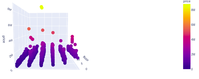
As you can see, the price increases and the number of rooms and floors increases.

Setting up the environment in PyCaret for regression data

The pycaret.regreesion is a supervised machine learning module is used for predicting continuous values/outcomes using various techniques and algorithms. It has over 25 algorithms and 10 plots to analyze the performance of models. Some of which we will explore in this section.

Now let us learn how to set up the environment for the PyCaret. The setup function initializes the environment in PyCaret and creates the transformation pipeline to prepare the data for modeling and deployment. It takes two mandatory parameters; the dataset and the target variable.

# Importing machine learning libraries pycaret
from pycaret.regression import *
# setting up machine learning workflows environment
Step = setup(data =Dushanbe, target = 'price', session_id=123)

Output:

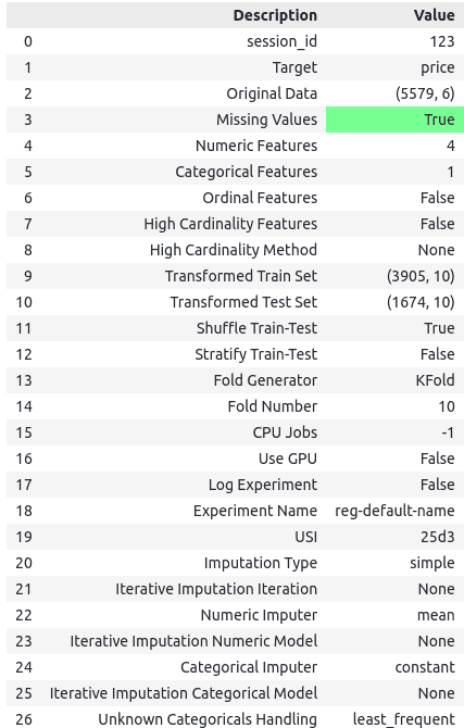
Once the setup has been successfully executed, it displays the information grid, which contains several important pieces of information. Most of the information is about the preprocessing of the data. Here we will discuss some of the preprocessing steps displayed above. Most of them are out of the scope of this article.

• Missing Values: It will be True if the data contains missing values. As we already had observed that our data had some missing values, it shows the missing values as True.
• Categorical Features: This shows the total number of features classified as categorical by the algorithm. In our case, it only identifies 1 feature to be categorical.
• Original Data: It shows the shape of the original data. In our case, the shape of the data is (5579, 6).
• Transformed Train Set: It shows the shape of the transformed training set. Notice that the original shape of (5579, 6) is transformed into (3905, 10) for the transformed train set. Due to categorical encoding, the number of features has increased from 6 to 10. That means the algorithm performs categorical encoding automatically as well.
• Transformed Test Set: It shows the shape of the transformed test data. In our case, the total shape of the testing set is (1674, 10). The splitting is performed based on a 70/30 ratio for training and testing. It can be changed by the train_size parameter while setting up the environment.

Comparing Regression models in PyCaret

The most important task of a Machine learning developer is to identify the best-fitting algorithm for the given dataset. One traditional way to select the best-fitted model is to use various algorithms and apply them to the given dataset. Then based on the performance evaluation, we can select the best model. But it is time consuming and might be difficult to implement some of the algorithms.

But the PyCaret compares the algorithm automatically and returns a list of models. The compare_models() method trains all models in the model library and scores them using k-fold cross-validation for metric evaluation. Then it prints a scoring grid that shows the average MAE, MSE, RMSE, R2, RMSLE, and MAPE. If you are unfamiliar with how these performance evaluation matrices are calculated, read about them from the implementation of linear regression using Python.

# automates machine learning workflows
best_models = compare_models()

Output:

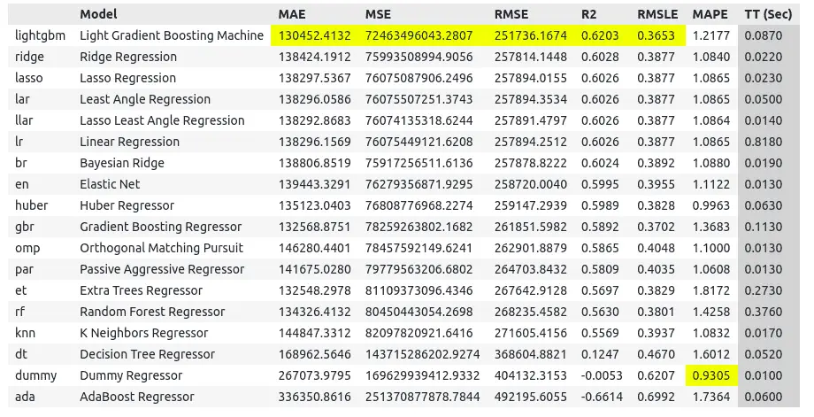
We have trained and evaluated nearly 20 Machine learning models using just one line of code. The scoring grid printed above highlights the highest-performing metric for comparison purposes. This shows that LightGBM performed well compared to all other algorithms.

The models are default sorted using the R2 score ( from highest to lowest). We can change the sorting by using the sort parameter. Also, the number of folds for the cross-validations is 10. We can also change it by using the fold parameter. Let us now change these parameters and compare different models again.

# train models 
best_models = compare_models(sort ='MAE', fold=5)

Output:

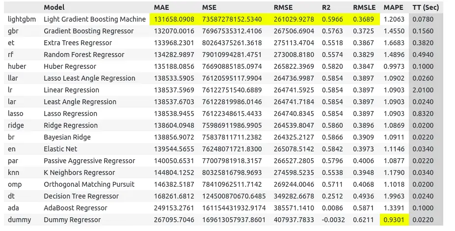
Notice that this time the models are sorted based on MAE values. N

We can now initialize any algorithms listed above using their ID values. Let us now jump into initializing models in PyCaret.

Creating and tunning regression model in PyCaret

Once we have a list of better-performing models, we can use any of them to train on our dataset. Training a model in PyCaret is much easier than using other Machine Learning techniques. In this section, we will train the model using the LightGBM algorithm. If you are unfamiliar with LightGBM, please look at the article implementation of LightGBM using Python.

The create_model() trains and evaluates a model using cross-validation. The output prints a scoring grid that shows MAE, MSE, RMSE, R2, RMSLE, and MAPE by fold. That means while using PyCaret. We don’t need to be worried about the evaluation of the model. It will be calculated automatically.

Let us use the create_mode() to create a LightGBM model.

# creating light gradient boosting machine model
LGBM = create_model('lightgbm')

Output:

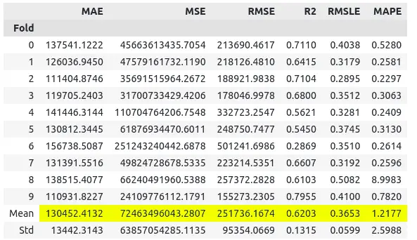
By default, the fold value is 10, so after 10 iterations, the model returns the means and standard deviation of each performance evaluation matrix. Looking at the R2 score, we can say that the model has performed pretty well, as it has a high value.

We can also print the model to see the default parameter values.

# printing the model parameters
print(LGBM)

Output:

These are the default parameter values that our model has been trained on.

Mostly, in model training, the hardest part is tuning the model. But PyCaret makes it so simple. We can tune the model by using just one line of code. The tuned_model() method is used for hyperparameter tuning. This automatically used the RandomGridSearch method to tune the model’s parameters on a pre-defined search space.

# automated hyperparameter tuning
LGBM_tunned = tune_model(LGBM)

Output:

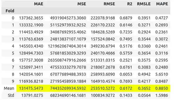
Now let us print the optimum parameter values that PyCaret has found.

These are the optimum parameters for the LightGBM model based on our dataset.

Plotting the regression model using PyCaret

Visualizations are the most important parts of training and predictions. Usually, we use different Python modules to visualize the results. But PyCaret helps us visualize the model using a few lines of code. And it also allows for plotting the model in various forms.

Let us first plot the residual plot of the model. Residual is the difference between the actual and the predicted values.

# Plotting the residual plot
plot_model(LGBM_tunned, plot='residuals')

Output:

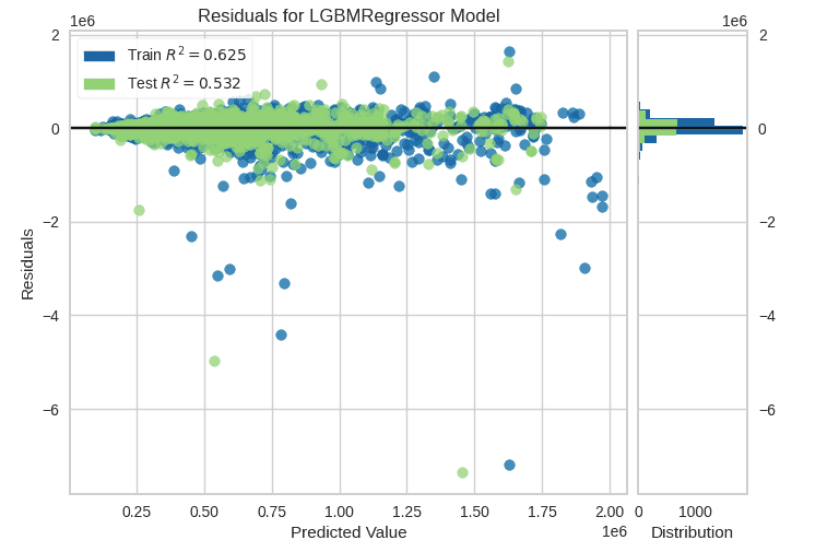
Apart from the residuals, the above plot also shows the distribution of the training and testing data predictions.

We can also plot the prediction error plot using only one line of code.

# Plotting the errpr plot
plot_model(LGBM_tunned, plot='error')

Output:

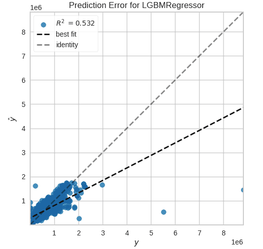
Notice that because of some outliers, our best-fitted line has tilted downward.

Using the same function, we can also visualize the feature’s importance as shown below:

# Plotting the feature importance
plot_model(LGBM_tunned, plot='feature')

Output:

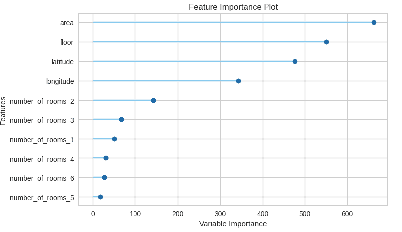
This shows that the area and number of floors are the most important features.

One more cool feature of PyCaret is that all the visualization and parameter tuning we did above can also be done using one line of code. The evaluate_model() function provides a user interface to plot various plots and perform hyperparameter tuning.

# model analysis
evaluate_model(LGBM_tunned)

Output:

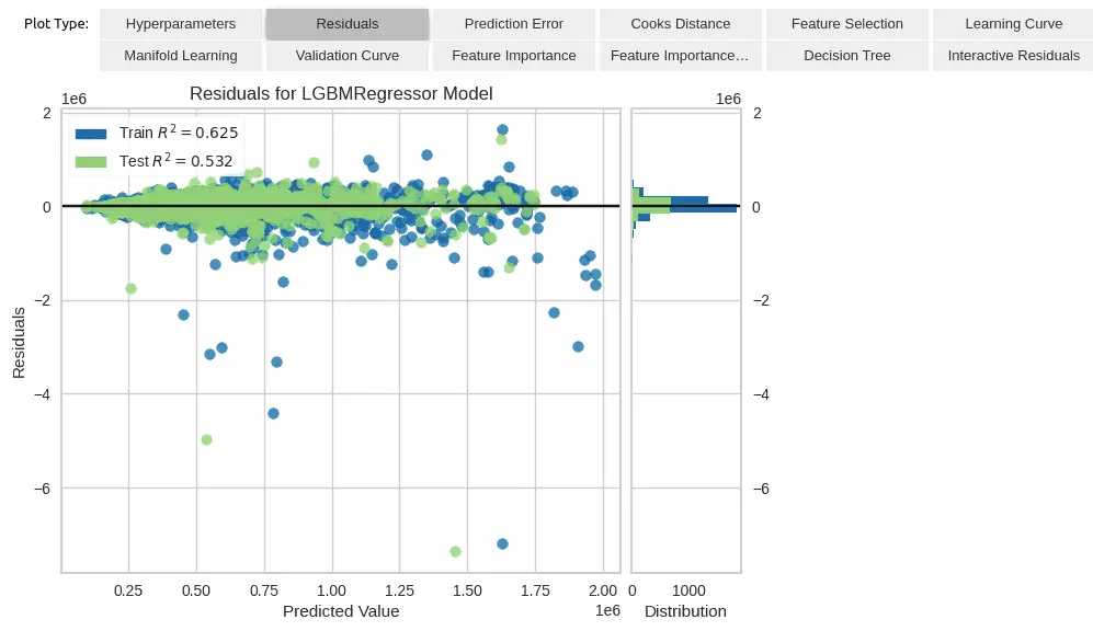
We can easily plot the graph by clicking on any of the above options.

Making predictions and saving the model

Notice that all the graphs we plotted above are based on the training dataset (70%). We didn’t use the testing data anywhere so far. We will use the testing data to make predictions and evaluate the model based on the testing dataset.

# predictions on new data
predict_model(LGBM_tunned)

Output:

Notice that we get an R2-score less than the previous one because, this time, the model is making predictions on the testing data, not the training dataset.

Once we are sure that the model is trained well and makes good predictions, we can save our model and use it later. The save_model() method takes two parameters, one the model and the second the name for the saving model.

# saving the model
save_model(LGBM_tunned,'LightGBM model for House priceing')

Once the model is saved, we will see a new file in the same directory where we are working. We can again load the model at any time using the load_model() and run in on a dataset.

# loading model
saved_model_lightgbm = load_model('LightGBM model for House priceing')

Once the model is loaded successfully, we can use it to make predictions.

Classification in Python using Pycaret

A dataset having categorical outputs is known as classification data. As we know, PyCaret is a module that uses built-in Machine learning algorithms smartly. So, before knowing how to implement the PyCaret on classification problems, make sure you have some knowledge of Machine learning algorithms that deal with classification problems.

The following classification algorithms are available in the PyCaret module.

• Ridge Classifier
• Logistic Regression
• Linear Discriminant analysis
• LightGBM
• Extra Tree classifier
• Support vector machine
• Naive Bayes
• Ada Boost Classifier
• K Neighbors classifier
• Dummy classifier
• Random forest classifier
• CatBoost classifier
• Decision Tree classifier
• Extra Trees classifier
• Extreme Gradient Boosting
• Gradient boosting classifier
• SVM – Linear kernel
• Quadratic Discriminant analysis

In this section, we will use the hear_disease data from the sub-module datasets. The dataset contains various input features affecting heart disease, and the output class contains binary values.

Importing and exploring the dataset

Let us now import the dataset and load it. In PyCaret, the get_dataa() method is used to load the dataset from the submodule.

# importing pycaret datasets module
from pycaret.datasets import get_data
# loading the dataset
heart_disease = get_data('heart_disease')

Output:

Notice that several features affect heart disease. Let us now see the total size of the dataset.

# shape of the dataset
heart_disease.shape

Output:

This shows that there are a total of 270 observations and 14 features. Let us also check if there are any null values in our dataset.

# missing values
heart_disease.isnull().sum()

Output:

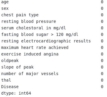
This shows that there are no null values in the dataset.

Setting up the environment in PyCaret for classification

Now we will use the setup() method to create an environment for the classification dataset.

# importing the pycaret for classification module
from pycaret.classification import *
# setup function
clf_model = setup(data = heart_disease, target = 'Disease')

Output:

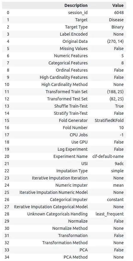
It returns all the details about the data and preprocessing steps. And also, notice that it has automatically split the data into testing and training parts.

Comparing the classification model in PyCaret

Once the module has created the environment, we can use the compare_models() method to return the list of best-fitted models.

# train models /model training
clf_best = compare_models()

Output:

This gives us a list of top models that best fit the dataset and their IDs. The models are sorted based on accuracy scores. Hence it is a binary classification problem, we will take logistic regression for further processing.

Creating a classification model in PyCaret

We will use create_model() method to create a logistic model. You can read about logistic regression in the article implementation of logistic-regression using Python.

# creating  model
LR = create_model('lr')

Output:

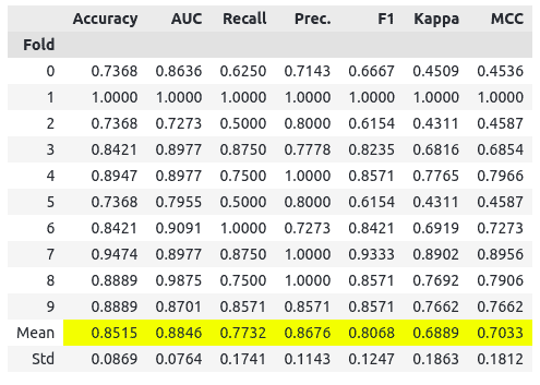
By default, the fold value is 10, which is why it stops after 10 iterations and gives the result with 85% accuracy. Let us print out the default parameter values.

# printing parameter values
print(LR)

Output:

These are the default values of the parameters, you can apply parameter tuning to get the optimum values as we did for the regression data.

Visualizing the classification model

The PyCaret module allows us to visualize the model in various ways. We will use some of the plotting features of the PyCaret to plot the trained model.

Let us plot the AUC graph for the trained model and an evaluation matrix for the classification dataset. The Area Under the Curve (AUC) measures the ability of a classifier to distinguish between classes and is used as a summary of the ROC curve. The higher the AUC, the better the model’s performance at distinguishing between the positive and negative classes. You can read more about AUC and ROC in this article,

# plotting AUC
plot_model(LR, plot = 'auc')

Output:

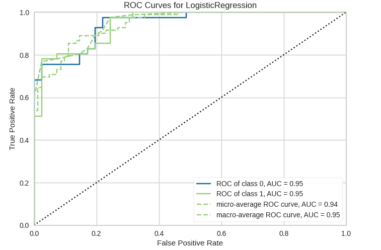
The AUC score is between 0.5-1. The higher the score is, the better the predictions are. In our case, the AUC score is 0.95, which is much higher.

One more cool feature of PyCaret is that we can plot a confusion matrix using just one line of code.

# plotting confusion matrix
plot_model(LR , plot = 'confusion_matrix')

Output:

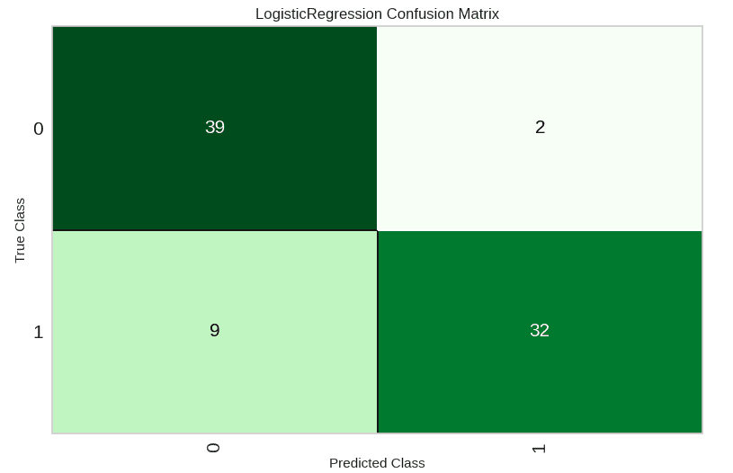
The confusion matrix shows that most of the 0 have been misclassified compared to 1.

Lastly, let us also plot the boundary to see the classification boundary.

# plotting boundary plot
plot_model(LR, plot = 'boundary', use_train_data = True)

Output:

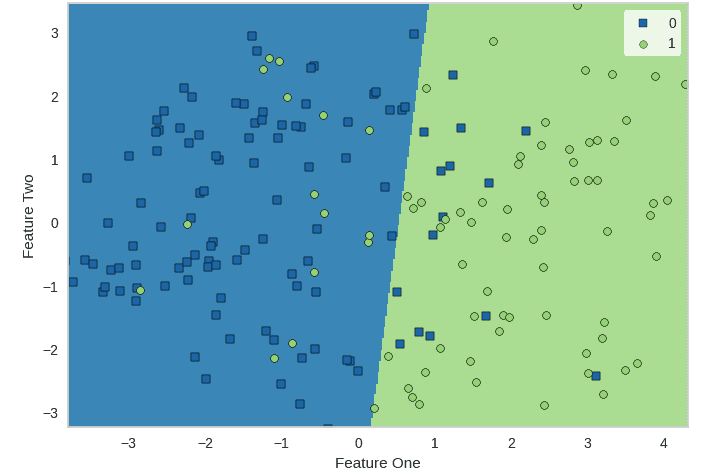
This shows the misclassified and correctly classified items visually.

Making predictions and saving model

As we have seen in the beginning, our data set was divided into testing and training parts, All the visualizations above were for the training dataset. We will use the testing data to make predictions and determine the accuracy score.

# making predictions
predict_model(LR)

Output:

Notice that the accuracy for the testing data is 86% which means 86% of the testing data was classified correctly.

Once we have finished training and testing the model, we can save it to use later without running the whole code easily.

# saving the model
save_model('LR', 'Logistic regression')

Once the model is saved, we can use it later by loading it as we did for the regression model.

Summary

PyCaret is an open-source and model management tool in Python that automates machine learning workflows. It contains 75+ algorithms and 25+ preprocessing techniques. It helps to compare, train, evaluate, tune, and deploy machine learning models with only a few lines of code. This article covered how we can use PyCaret to create regression and classification models and visualize the results.